Tutorial A13 – Solutions

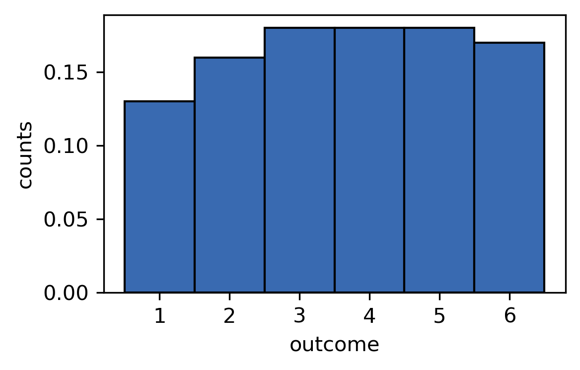
1 Modify the coinflip section from lesson A13 to simulate throwing a dice. Throw the dice 100 times and save the outcomes \(X_i\) with \(i = 1, ... , N\) in a list. Plot the result as a histogram.

import matplotlib as mpl
import matplotlib.pyplot as plt
import numpy as np
import random


mpl.rc_file(
    "../../matplotlibrc",
    use_default_template=False
)

random.seed(1)

def throw_n_times(n):
    """Throw a dice n times

    Returns:
        List of outcomes
    """

    throws = []  # Outcomes
    for _ in range(n):
        # Draw a random number
        random_number = random.random()

        # We want all outcomes to be equally likely
        # The following lines assign the random number to either outcome

        # Integer just truncated after the decimal point is used like the ceil function here
        outcome = int(random_number * 6 + 1)

        # Finally, store the outcome
        throws.append(outcome)
    return throws

throws = throw_n_times(100)
plt.hist(throws, bins=[0.5, 1.5, 2.5, 3.5, 4.5, 5.5, 6.5], density=True, edgecolor='k')
plt.xticks((1, 2, 3, 4, 5, 6))
plt.xlabel('outcome')
plt.ylabel('counts')

Text(0, 0.5, 'counts')

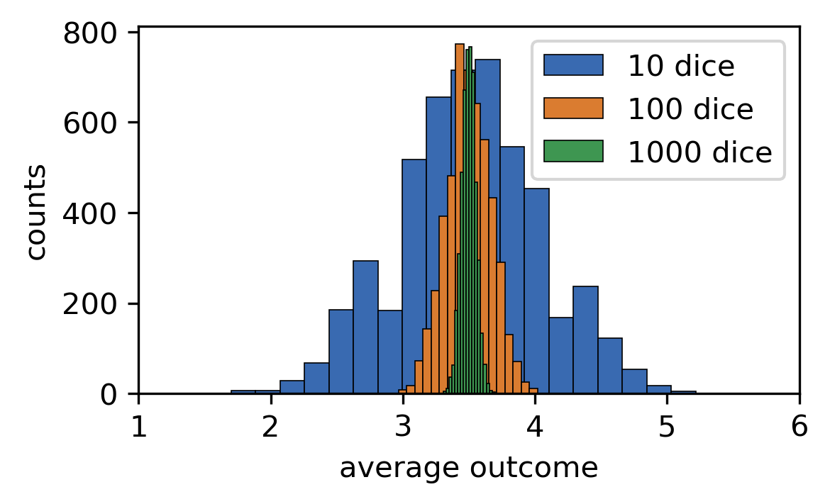
2 Modify the code further to throw \(N = 10, 100, 1000\) dice and store the mean values \(S_N = \frac{1}{N}\sum_{i=1}^N X_i = \langle X \rangle\) in a list. For each \(N\) repeat the experiment 5000 times and plot the resulting distributions of mean values.

random.seed(2020)

plt.figure()
random.seed(2020)

for n in [10, 100, 1000]:
    mean_values = []

    for t in range(5000):
        throws = throw_n_times(n)
        m = sum(throws) / n
        mean_values.append(m)

    plt.hist(mean_values, 20, label=f'{n} dice', edgecolor='k', linewidth=0.4)

plt.legend()
plt.ylabel('counts')
plt.xlabel('average outcome')
plt.xticks((1, 2, 3, 4, 5, 6))
plt.tight_layout()

3 Repeat the experiment of task 2 but instead of plotting the distribution of mean values \(S_N\), plot the distribution of \(\sqrt{N}(S_N - \mu)\), where \(\mu\) is the expectation value \(\mu = \frac{1}{M}\sum_k^M w_k X_k\), where \(\omega_k\) and \(X_k\) are the weights and possible outcomes of the random variables, respectively. In the case of a dice the expectation value is \(\mu = (1 + 2 + 3 + 4 + 5 + 6) / 6 = 3.5\). What do you observe?

random.seed(2020)

plt.figure()

for n in [10, 100, 1000][::-1]:
    mean_values = []

    for t in range(5000):
        throws = throw_n_times(n)
        m = np.sqrt(n) * (sum(throws) / len(throws) - 3.5)
        mean_values.append(m)

    plt.hist(mean_values, 20,
             label=f'{n} dice',
             edgecolor='k', linewidth=0.4)

plt.legend()
plt.ylabel('counts')
plt.xlabel('outcome')
plt.tight_layout()

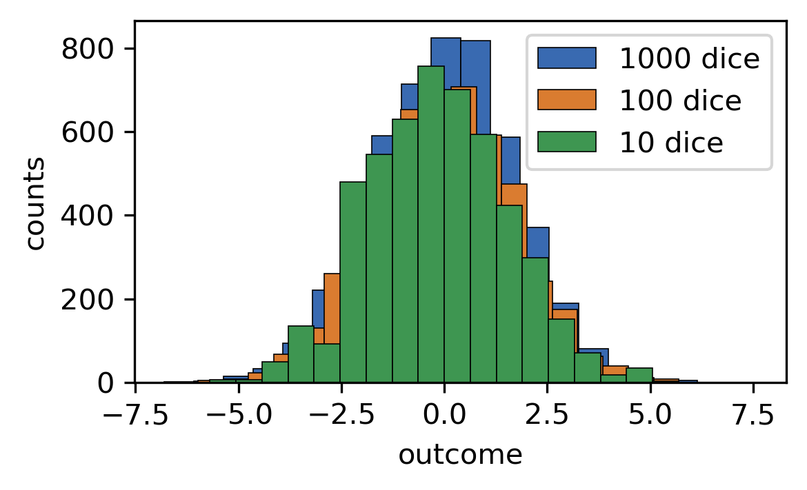
The distributions converge towards mean-zero normal distributions. This is a manifestation of the central limit theorem, which states that the \(\mu\)-shifted average values of an increasing sample size converge towards a normal distribution with variance \(\sigma^2 = \langle (X-\mu)^2 \rangle\)

\[\lim_{N->\infty}\sqrt{N}(S_N-\mu)=\mathcal{N}(0,\sigma^2)\]

((np.arange(1, 7) - 3.5)**2).mean()

2.9166666666666665