Lesson A13 – Random numbers

The random module

The random module in the Python standard library contains the Python random number generator (RNG) and some related functionality. Refer to the official documentation for anything we are not covering in this tutorial. As we will see, the generation of random numbers is not only nice for illustration purposes. Import the module like this:

import random

The module has two fundamental functions: random.seed() and random.random(). The first sets the seed (the origin) for the RNG. The second draws a sequence of uniformly distributed random numbers in the half-open interval \([0, 1)\). The results differ with each execution of random.random() depending on the seed. This becomes a problem if one wants reproducible results, e.g. for debugging. Setting a seed fixes this problem.

The seed determines the produced sequence of random numbers. So fixing the seed makes the RNG return random numbers that are predictable (which sounds admittedly paradox). This is demonstrated below. We set the seed to zero and print the first five random numbers. Repeating the process three times yields identical sequences, always. This is useful for creating reproducible results that rely on random numbers.

for _ in range(3):
    print("Seed = 0")
    random.seed(a=0)
    for i in range(5):
        print(i + 1, random.random())
    print()

Seed = 0
1 0.8444218515250481
2 0.7579544029403025
3 0.420571580830845
4 0.25891675029296335
5 0.5112747213686085

Seed = 0
1 0.8444218515250481
2 0.7579544029403025
3 0.420571580830845
4 0.25891675029296335
5 0.5112747213686085

Seed = 0
1 0.8444218515250481
2 0.7579544029403025
3 0.420571580830845
4 0.25891675029296335
5 0.5112747213686085

Further functionality, derived from the basic random.random() function, includes:

• random.randrange(start, stop, step): returns a random element of range(start, stop, step)

• random.randint(a, b): returns a random integer from the interval [a, b]

• random.choice(seq): returns a random element from a sequence

• random.choices(seq, k=1): returns a list of k random elements from a sequence (with replacement)

• random.sample(seq, k): returns a list of k random elements from a sequence (without replacement)

• random.shuffle(seq): shuffles a sequence in-place (brings the elements in randomly different order)

x = list(range(10))
print("Before shuffling x =", x)
random.shuffle(x)
print("After  shuffling x =", x)
print("Random samples:     ", random.sample(x, 3))
print("Random choices:     ", random.choices(x, k=3))
print("Random choice:       ", random.choice(x))

Before shuffling x = [0, 1, 2, 3, 4, 5, 6, 7, 8, 9]
After  shuffling x = [9, 0, 3, 5, 1, 8, 2, 7, 4, 6]
Random samples:      [0, 1, 3]
Random choices:      [5, 7, 4]
Random choice:        8

Note: Note that shuffle does not return a shuffled list but changes the passed sequence in-place.

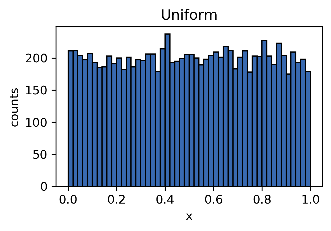
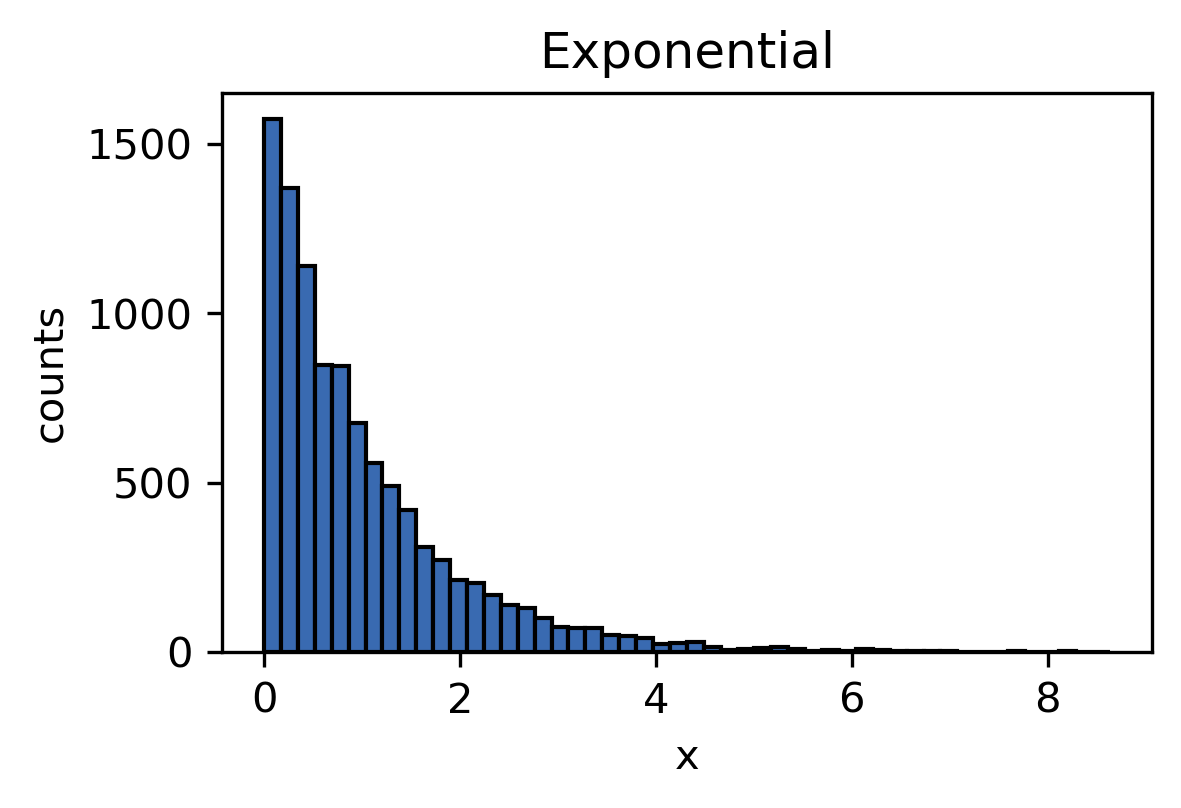
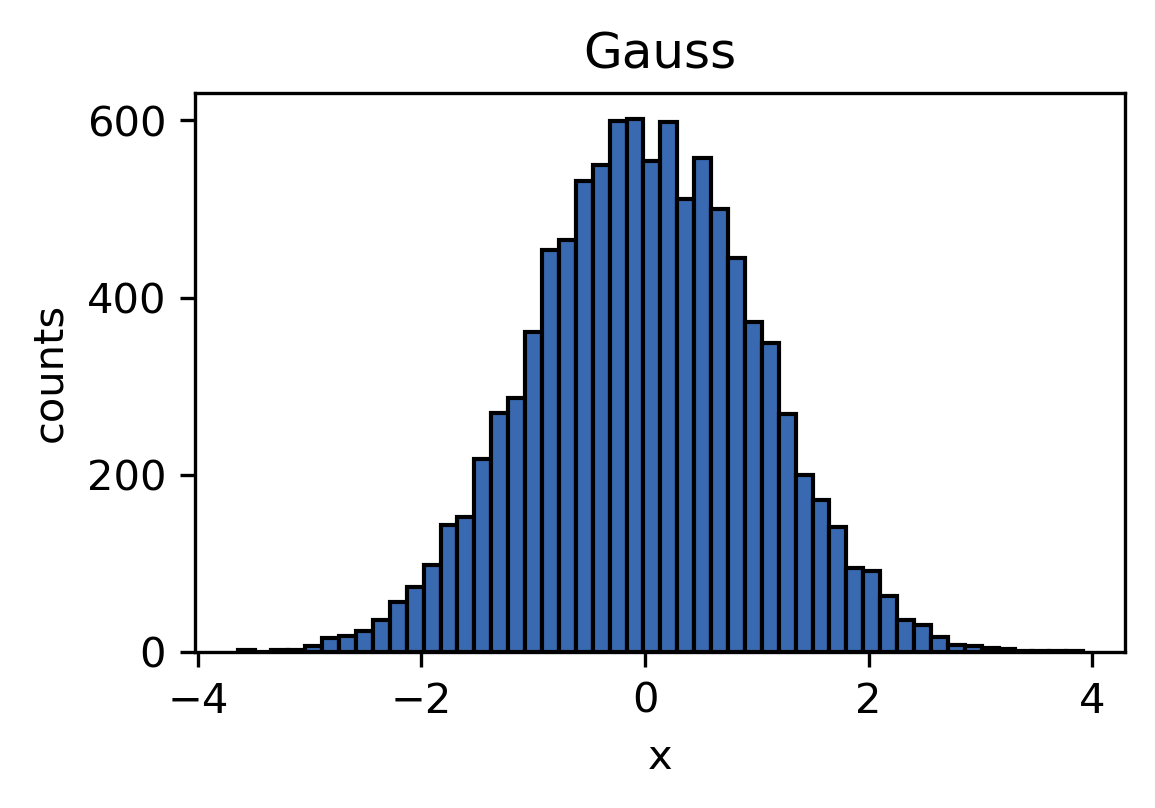
Several distributions to draw random numbers from are implemented as well. The available distributions are shown for 10000 sample points each below. We are using matplotlib to show example plots.

import matplotlib as mpl
import matplotlib.pyplot as plt

mpl.rc_file(
    "../../matplotlibrc",
    use_default_template=False
)

def test_rand(func, title, *args, **kwargs):
    """Helper funtion to demonstrate sample distributions.

    Draws a number of samples with a given function and displays
    the collection of samples as histogram.

    Args:
        func: function to sample from.
        title: title used for the plot
        *args, **kwargs: passed on to `func`
    """

    x = []
    n = 10000  # number of samples

    for _ in range(n):
        x.append(func(*args, **kwargs))

    plt.figure()
    plt.hist(
        x, 50,
        edgecolor="k"
        )
    plt.xlabel("x")

    plt.ylabel("counts")
    plt.title(title)

Advanced: Have you noticed the starred arguments *args and **kwargs in the definition of our helper function? We use *args when we want allow to pass an arbitrary number of positional arguments to a function. In this case we use it to pass possibly passed arguments to test_rand() further on to the function func. Note that args as a name is just a convention. The star in front of it makes all positional arguments beyond func and title be stored in a list args (args = [arg1, arg2, ...]). The same goes for keyword arguments and **kwargs. For keyword arguments, however, the double star makes all passed keyword arguments be stored in a dictionary (kwargs = {kwarg: value, ...}).

# Definition of call signatures
# (func, name, args, kwargs); Note that we actually only use args
calls = [
    (random.uniform, "Uniform", [0, 1], {}),
    (random.expovariate, "Exponential", [1], {}),
    (random.gauss, "Gauss", [0, 1], {}),
# Other distributions:
#   (random.gammavariate, "Gamma", [1, 1], {}),
#   (random.triangular, "Triangular", [0, 1], {}),
#   (random.betavariate, "Beta", [1, 2], {}),
#   (random.lognormvariate, "Log normal", [0, 1], {}),
#   (random.vonmisesvariate, "Von Mises", [0, 1], {}),
#   (random.paretovariate, "Pareto", [10], {}),
#   (random.weibullvariate, "Weibull", [1, 1], {}),
    ]

for call_ in calls:
    print(call_)
    test_rand(call_[0], call_[1], *call_[2], **call_[3])

(<bound method Random.uniform of <random.Random object at 0x5643c4c8ffa8>>, 'Uniform', [0, 1], {})
(<bound method Random.expovariate of <random.Random object at 0x5643c4c8ffa8>>, 'Exponential', [1], {})
(<bound method Random.gauss of <random.Random object at 0x5643c4c8ffa8>>, 'Gauss', [0, 1], {})

Other Distributions are available as well but not shown. You can choose to plot them by uncommenting the respective line above. They depend on one or two paramters that have to be chosen within a specifc range. For more details, use help(random.foo) where you replace foo with the distribution you are curious about.

Coinflip

We can use RNGs to simulate random processes like flipping a coin. We assign the outcomes heads and tails to the values of 0 and 1, respectively.

# Create a figure
plt.figure()

j = 0
# subplot index

# Try different numbers of coin throws
for n in [20, 200, 2000, 20000]:
    throws = []  # Store the outcomes in this list

    # Throw the coin n times
    for i in range(n):
        # Draw a Random Number
        random_number = random.random()

        # We want both outcomes to be equally likely
        # The following lines assign the random number to either outcome
        if random_number < 0.5:
            outcome = 1
        else:
            outcome = 0

        # finally, store the outcome
        throws.append(outcome)

    # Plotting section
    j += 1  # Increase subplot index
    plt.subplot(2, 2, j)  # Add subplot
    plt.hist(throws, 2, edgecolor='k')
    plt.title(f'{n} throws', fontsize="small")
    plt.ylabel('counts', fontsize="small")
    plt.xticks(
        ticks=[0.25, 0.75],
        labels=['heads', 'tails'],
        fontsize="small"
        )
    plt.yticks((0, n), fontsize="small")

plt.subplots_adjust(hspace=0.6, wspace=0.6)

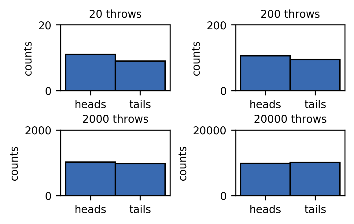
As expected, the number of counts for both outcomes converges to the same value for an increasing number of throws.

Advanced

Monte Carlo Simulations

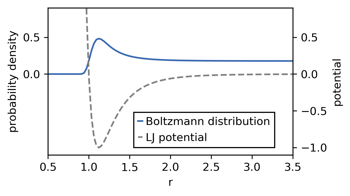
Monte-Carlo simulations are used when one cannot (efficiently) sample the probability density function, e.g. the Boltzmann distribution in high-dimensional spaces. This section illustrates the Metropolis-Monte-Carlo algorithm to sample the Boltzmann distribution of the Lennard-Jones potential.

Note: You can in principle use the a Monte-Carlo approach to draw samples from any given probability distribution (see earlier mentioned examples). In practice the above distributions are probably generated by the cumulative distribution function (CDF), though.

All one needs, is a random number generator, that generates uniformly distributed random numbers to achieve this goal. Lets try to draw samples from the distribution shown below, which is a Boltzmann distribution corresponding to a 12-6 Lennard-Jones potential with arbitrarily chosen parameters (\(\epsilon = 1\), \(\sigma = 1\)). We want to generate a sequence of samples following this distribution, in other words sample configurations in the underlying potential. Note that we use the NumPy module for convenience.

import numpy as np

def V(x):
    """LJ potential"""

    return 4*((1./x)**12 - (1./x)**6)

r = np.linspace(0.01, 6, 200)

beta = 1.0  # Temperatur factor
v = V(r)
bmd = np.exp(-beta * v)
q = np.trapz(bmd, r)  # Partition function
bmd /= q

fig, axd = plt.subplots()
axv = axd.twinx()
dline = axd.plot(r, bmd)
vline = axv.plot(r, v, color="gray", linestyle="--")
axd.set_xlabel('r')
axd.set_ylabel('probability density')
axv.set_ylabel('potential')
axd.set_yticks((0, 0.5))
axd.set_xlim(0.5, 3.5)
axd.set_ylim(-1.1, 0.9)
axv.set_ylim(-1.1, 0.9)
axd.legend(
    [dline[0], vline[0], ],
    ["Boltzmann distribution", "LJ potential",],
    fancybox=False,
    framealpha=1,
    edgecolor="k",
    loc=(0.35, 0.05),
    handlelength=0.4,
    handletextpad=0.3
)

<matplotlib.legend.Legend at 0x7f57889f2048>

Lets switch to NumPy’s random module for the random number generation. The functionality is similar to that of the lightweight standard library module, but offers a bit more. It is also possible to obtain sequences of generated numbers directly as numpy arrays. Another advantage lies in the fact that the numpy implementation tries to do a lot of the computation actually in C, which can be faster and more efficient when you want to generate large amounts of numbers.

Lets set a good seed to get lucky with the random numbers.

np.random.seed(666)

The Metropolis-Hastings algorithm works as follows. We initialise the sequence of random samples by choosing a starting sample (configuration). Then we make a step away from this configuration, i.e. we choose a possible next sample. We accept this possible next sample as the actual next sample according to the relative probabilities of the current and the possible next sample in question. We obtain the relative probabilities from the distribution we want to draw from. In more mathematical terms we do:

• choose a trial sample : \(x_{\mathrm{trial}} = x_n + \delta\)

• compute the acceptance ratio: \(p_{\mathrm{accept}}= \min \left(1, \frac{p( x_\mathrm{trial})} { p(x_n)} \right) = \min(1, \exp(-\beta\left( V(x_\mathrm{trial}) - V(x_n) \right)\)

• next draw a uniformly distributed random number \(q\) and if \(q < p_\mathrm{accept}\) set \(x_{n+1} = x_\mathrm{trial}\), else the trial step is rejected and another trial step needs to be chosen

It is important that \(\delta\) is drawn from a mean-zero distribution, such that it can take negative and positive values with equal probability. Otherwise one needs to account for the asymmetry in choosing a trial step by including additional terms into the acceptance ratio. The size of \(\delta\) can be tuned with scalar factors.

So let’s look at a possible realisation of this. We use the scheme to draw different amounts of samples and compare the sampled distribution with the analytic one.

x = 0.8  # Initial configuration
alpha = 0.02  # Delta scale factor

samples = []  # sample container
samples.append(x)

for _ in range(500000):
    step = alpha * 2 * (np.random.rand() - 0.5)
    # draw delta from uniform distribution [-1, 1) (scaled by alpha)

    x = samples[-1] + step  # Trial sample
    dE = V(x) - V(samples[-1])  # Energy difference between current and trial
    pa = np.exp(-beta * dE)  # Probability ratio

    coin = np.random.rand()  # Do we accept?
    if coin >= pa:
        continue
    samples.append(x)

for i in [1000, 5000, 10000, 50000, 100000, 500000]:
    plt.figure(
        figsize=(
            mpl.rcParams["figure.figsize"][0],
            mpl.rcParams["figure.figsize"][1] * 0.4
            )
        )

    hist = plt.hist(
        samples[:i],
        bins=50,
        density=True,
        edgecolor="k",
        label=f"{i} samples",
        )
    plt.plot(
        r, bmd,
        color='#cc2529',
        linewidth=2,
        label='analytical solution'
        )

    plt.ylabel('density')
    plt.xlim(min(hist[1])*0.9, max(hist[1])*1.1)
    plt.xlabel('r')
    plt.legend(
        fancybox=False,
        framealpha=1,
        edgecolor="k",
        loc=0,
        handlelength=0.4,
        handletextpad=0.5,
        fontsize="small"
        )

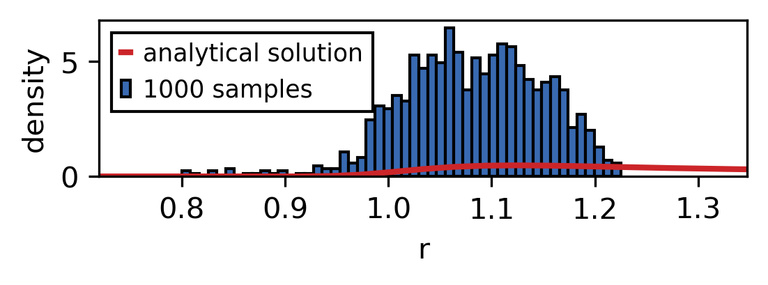
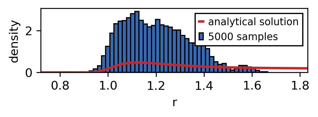
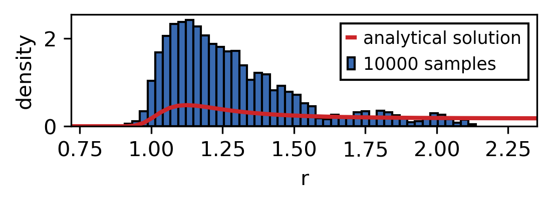
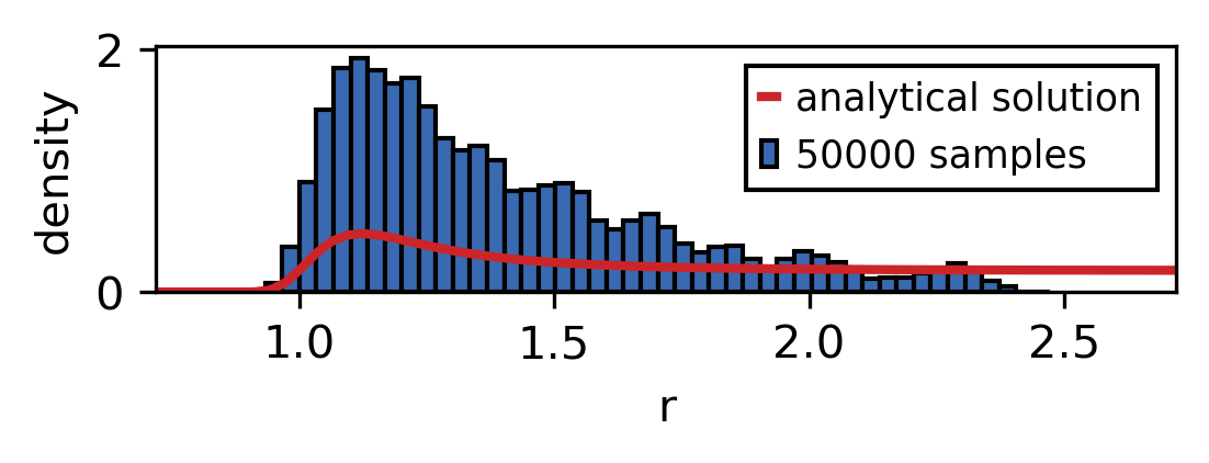
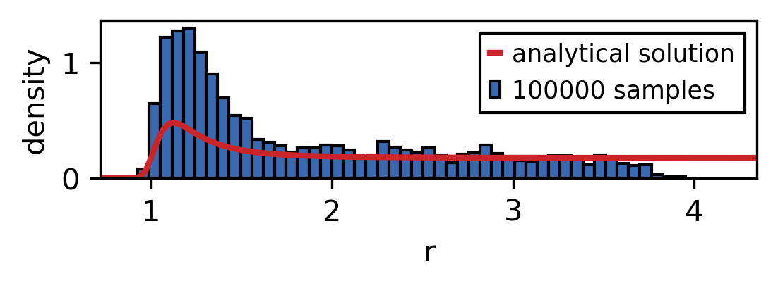
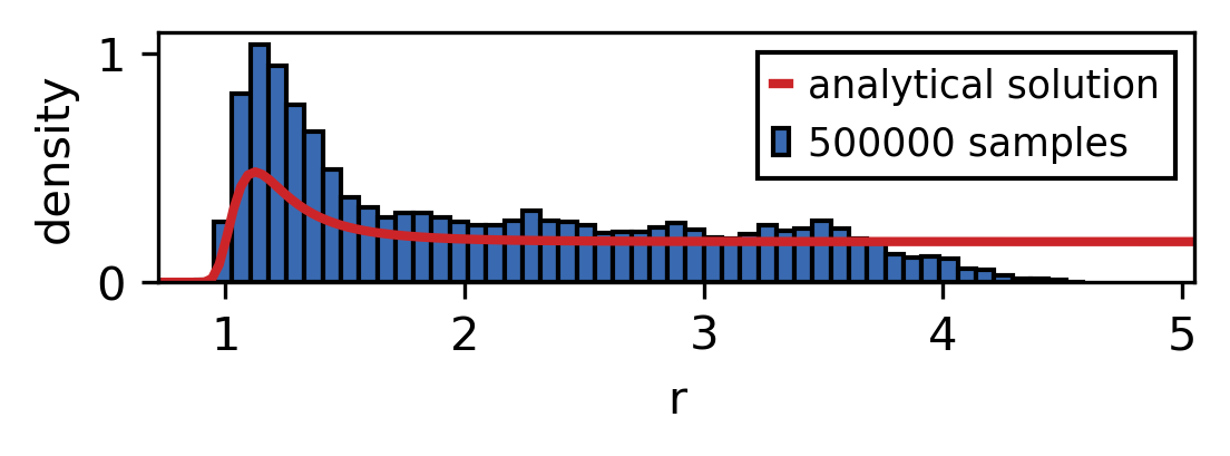
As the sample size is increased the sampled distribution converges towards the analytical solution. As you can see the convergence is rather slow and the analytical solution is never recreated perfectly. However longer simulation times also mean that larger parts of the phase space are explored.

Random walks

The sequence of samples generated by the Metropolis-Monte Carlo scheme is not a trajectory in time because the way we generated the trial configurations has no connection to the time involved to make the corresponding step. We could make very big or very small changes to system (or no change at all) with equal probability within one step (\(\delta\) was drawn from a uniform distribution). So while the static distribution of samples has a physical meaning, the actual dynamic sequence of samples has not. The pseudo-dynamic step trajectory can, however, be considered a random walk.

plt.figure(
    figsize=(
        mpl.rcParams["figure.figsize"][0],
        mpl.rcParams["figure.figsize"][1] * 0.4
        )
    )
plt.plot(samples)
plt.xlabel('step')
plt.ylabel('r')
plt.xlim(0, len(samples))

(0, 496061)

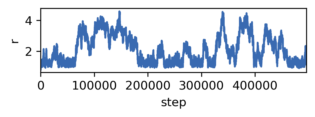
The series of r changes in random increments and discretely in “time”. We call such a process a random walk. Random Walks are stochastic processes in discrete time with stationary increments. A random walk can be defined as follows:

Let \((Z_1,Z_2,...,)\) be random numbers of the same underlying distribution. Then

\(X_n = x_0 + \sum_{i=1}^n Z_i, n\in \mathbb{N}\)

defines the random walk. \(x_0\) is the starting point and usually chosen to be 0.

Although the series of sample points carries no physical meaning, ensemble properties in physics can be accurately described with random walks. As an example of this, choosing a normal distribution to be the underlying distribution results in a Wiener process, a mathematical model for Brownian motion.

def generate_rw(n, t, alpha):
    """Generate N random walks consisting of T steps.

    The stepsize lies in the interval (-alpha, alpha].

    Args:
        n (int): The number of random walks to be generated

        t (int): The number of steps per random walk

        alpha (float): The maximum size of one step

    Returns:
        Array of shape (t, n) where X[:, i] is the ith random walk.
    """

    return np.cumsum(
        2. * alpha * (np.random.uniform(size=(t, n)) - 0.5),
        axis=0
        )

n = 10
t = 100
X = generate_rw(n, t, 3)
plt.plot(X)
plt.xlabel('step')
plt.ylabel('x')
plt.xlim(0, t)

(0, 100)

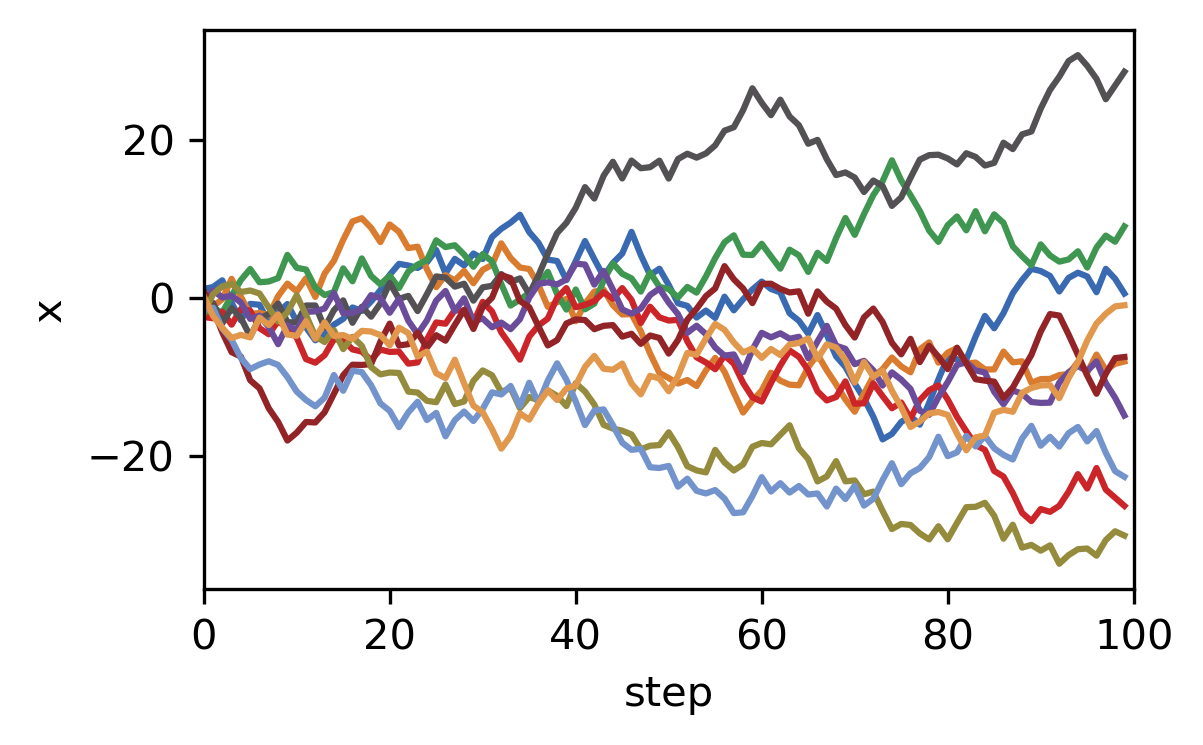
As you can see, with NumPy we can easily generate several random walks of any length in a single statement.