![]()
AlgoSB 2021
Practical afternoon session Monday, 8th of November. Time-series analysis, covering:
Principle component analysis
Time-lagged independent analysis
Clustering
MSM estimation
[1]:
from dataclasses import dataclass
import sys
import warnings

import cnnclustering
from cnnclustering import cluster
from IPython.core.display import display, HTML
import  matplotlib as mpl
import matplotlib.pyplot as plt
import numpy as np
import pyemma
import scipy
from scipy.stats import multivariate_normal
import sklearn
import sklearn.decomposition
import sklearn.cluster
Optional dependency module not found:  No module named 'networkx'
Optional dependency module not found:  No module named 'networkx'
[2]:
# Jupyter display settings
display(HTML("<style>.container { width:90% !important; }</style>"))
[3]:
# Version information
print("Python: ", *sys.version.split("\n"))

print("Packages:")
for package in [mpl, np, scipy, sklearn, pyemma, cnnclustering]:
    print(f"    {package.__name__}: {package.__version__}")
[4]:
# Matplotlib configuration
mpl.rc_file(
    "../matplotlibrc",
    use_default_template=False
)
[5]:
warnings.simplefilter("ignore")
Motivation
[6]:
%%HTML
<video width="90%" src="motivation.mp4" controls></video>
Outline and organisation
We will demonstrate a few types of analyses that can be used in Markov-model estimation workflows on Molecular Dynamics data. Instead of “real world” MD trajectories, we will use artificial time-series that we produce as follows:
We define a transition-probability matrix for a number of (conformational) states. An element \(ij\) in this matrix denotes the observation probability for a (conformational) transition from state \(i\) to state \(j\) within a time-step.
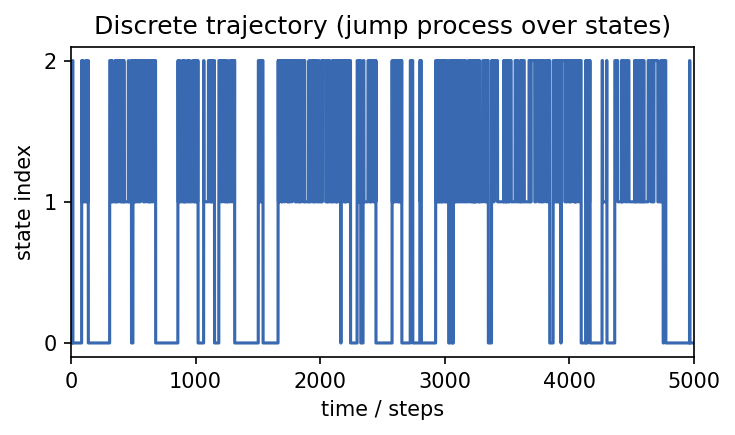
Starting from this matrix, we generate a possible time-series in state space, i.e. a discrete trajectory, which reflects the given transition probabilities.
Next, we define our states in terms of underlying probability distributions in a feature space (e.g. multivariate gaussians).
For each time-step in the discrete time-series, we draw a (conformational) sample from the distribution of the corresponding state to generate a continuous trajectory
The continuous trajectory (conformational snapshots in the feature space) are subjected to different analyses.
Note: In a “real” analysis we would proceed basically the other way round. Starting from a trajectory trough a continuous feature space obtained by a MD simulation, we want to produce a discrete trajectory (e.g. trough clustering) to finally estimate a transition probability matrix that describes our system.
To organise the “systems” we investigate in this exercise, let’s use a simple wrapping object to collect everything a system is made of:
[7]:
@dataclass
class System:
    desc: str
    transition_p_matrix: np.ndarray = None
    dtraj: np.ndarray = None
    state_distr_map: dict = None
    traj: np.ndarray = None
    pca=None
    tica=None
    clustering_commonnn=None
    clustering_voronoi=None
Data set generation
[8]:
system_intro = System("Introductory example")
system = system_intro
Transition probability matrix and time-series over states
\(p_{ij}\): Probability that the system is in state \(j\) at time \(t + \tau\) after being in state \(i\) at time \(t\).
[9]:
# Arbitrary transition probabilities for three states
system.transition_p_matrix = np.array([
    [0.98, 0.00, 0.02],
    [0.00, 0.89, 0.11],
    [0.02, 0.11, 0.87],
])
[10]:
# Dummy MSM from transition probabilities
sampled_msm = pyemma.msm.SampledMSM(system.transition_p_matrix)
system.dtraj = sampled_msm.simulate(5000)
[11]:
system.dtraj[:30]
[11]:
array([0, 0, 0, 0, 0, 0, 0, 0, 0, 0, 0, 2, 2, 2, 0, 0, 0, 0, 0, 0, 0, 0,
       0, 0, 0, 0, 0, 0, 0, 0])
[12]:
fig, ax = plt.subplots()
line, = ax.plot(system.dtraj)
ax.set(**{
    "title": "Discrete trajectory (jump process over states)",
    "xlabel": "time / steps",
    "ylabel": "state index",
    "xlim": (0, len(system.dtraj)),
    "yticks": np.unique(system.dtraj)
})
fig.tight_layout()
Probability distributions for states in feature space
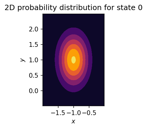
Let’s assume we know for each state a corresponding probability distribution in a \(k\)-dimensional conformational space \(\mathbb{R}^k\). For example, let’s model each state by a multivariate Gaussian with center \(\mu\) and covariance matrix \(\Sigma\):
[13]:
# Three states in 2D
state_centers = np.array([
    [-1, 1],
    [1, -1],
    [2, 2],
])
state_covs = np.array([
    [[0.1, 0.0],
     [0.0, 0.3]],
    [[0.4, 0.0],
     [0.0, 0.4]],
    [[0.2, 0.0],
     [0.0, 0.2]],
])
[14]:
def make_state_distributions(centers, covs):
    """Create a mapping of state IDs to gaussian distributions"""

    return {
        index: multivariate_normal(mean=center, cov=cov)
        for index, (center, cov) in enumerate(zip(centers, covs))
    }
[15]:
system.state_distr_map = make_state_distributions(state_centers, state_covs)
[16]:
# Draw a random point from a state distribution
system.state_distr_map[0].rvs()
[16]:
array([-1.17546117, 0.47576218])
[17]:
x, y = np.mgrid[-1.99:0:.01, -0.49:2.5:.01]
pos = np.dstack((x, y))

state_index = 0

fig, ax = plt.subplots()
ax.contourf(
    x, y, system.state_distr_map[state_index].pdf(pos),
    cmap=mpl.cm.inferno
)
ax.set(**{
    "aspect": "equal",
    "title": f"2D probability distribution for state {state_index}",
    "xlabel": "$x$",
    "ylabel": "$y$",
})
fig.tight_layout()
Continuous trajectory through feature space
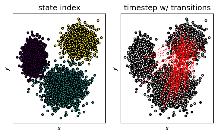
Now we can translate the discrete trajectory through state space into a (randomised) continuous trajectory in feature space.
[18]:
def sample_trajectory_from_discrete(dtraj, mapping):
    """Map discrete state trajectory to random conformational samples"""
    return np.array([
        mapping[state].rvs()
        for state in dtraj
    ])
[19]:
system.traj = sample_trajectory_from_discrete(
    system.dtraj,
    system.state_distr_map
)
[20]:
def get_transition_points(dtraj):
    """Determine state transition points in discrete trajectory"""

    inter_state_transitions = []

    for i, state in enumerate(dtraj[1:]):
        last_state = dtraj[i]

        if state != dtraj[i]:
            inter_state_transitions.append(i)

    return inter_state_transitions
[21]:
fig, (state_ax, time_ax) = plt.subplots(1, 2)
state_ax.scatter(
    *system.traj.T,
    c=system.dtraj,
    s=10,
    edgecolors="k", linewidths=1
)
time_ax.scatter(
    *system.traj.T,
    c=np.arange(system.traj.shape[0]),
    s=10,
    edgecolors="k", linewidths=1,
    cmap=mpl.cm.gray
)

for i in get_transition_points(system.dtraj):
    if i % 5 != 0:
        continue
    start = system.traj[i]
    end = system.traj[i + 1]
    time_ax.plot(
        [start[0], end[0]], [start[1], end[1]],
        color="red", linestyle="dotted", linewidth=1,
    )

for ax in (state_ax, time_ax):
    ax.set(**{
        "aspect": "equal",
        "xticks": (),
        "yticks": (),
        "xlabel": "$x$",
        "ylabel": "$y$"
    })

state_ax.set_title("state index")
time_ax.set_title("timestep w/ transitions")

fig.tight_layout()
Exercise
Use the described scheme to generate your own toy data set, starting from a self-defined transition probability matrix (e.g. four states in 3D).
Principle component analysis
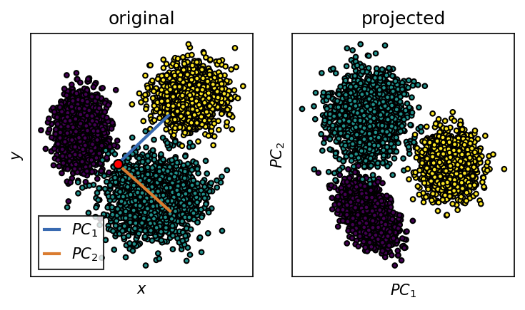
We want to use PCA to transform the input coordinates into a new set of meaningful coordinates. After PCA, the first obtained coordinate (\(PC_1\)) is aligned with the axis of maximum variance in the input space.
[25]:
system = system_intro
[26]:
# Do PCA
system.pca = sklearn.decomposition.PCA(n_components=2)
system.pca.fit(system.traj)
[26]:
PCA(n_components=2)
[27]:
# Obtained principle components (n_component, n_dim)
components = system.pca.components_
components
[27]:
array([[ 0.69673861,  0.71732511],
       [ 0.71732511, -0.69673861]])
[28]:
# Project original trajectory into PC-space
projected_trajectory = system.pca.transform(system.traj)
[29]:
# How much information is entailed in the PCs?
system.pca.explained_variance_ratio_
[29]:
array([0.55057159, 0.44942841])
[30]:
fig, (o_ax, p_ax) = plt.subplots(1, 2)
o_ax.scatter(
    *system.traj.T,
    c=system.dtraj,
    s=10,
    edgecolors="k", linewidths=1
)

scale = 2  # Scale PC vectors by this factor
o_ax.plot([0, components[0, 0] * scale], [0, components[0, 1] * scale], linewidth=2)
o_ax.plot([0, components[1, 0] * scale], [0, components[1, 1] * scale], linewidth=2)
o_ax.plot([0], [0], markerfacecolor="red", marker="o", markeredgecolor="k")

p_ax.scatter(
    *projected_trajectory.T,
    c=system.dtraj,
    s=10,
    edgecolors="k", linewidths=1
)
o_ax.set(**{
    "xticks": (),
    "yticks": (),
    "xlabel": "$x$",
    "ylabel": "$y$",
    "title": "original"
})

p_ax.set(**{
    "xticks": (),
    "yticks": (),
    "xlabel": "$PC_1$",
    "ylabel": "$PC_2$",
    "title": "projected"
})

o_ax.legend(
    ["$PC_1$", "$PC_2$"],
    handlelength=1,
    fancybox=False,
    edgecolor="k"
)

fig.tight_layout()
Exercise
Use sklearn.decomposition.PCA to perform a principle component analysis on your own data set. Visualize the obtained components and the trajectory projected onto the first two of them. How much of the total variance in the data set is explained by the PCs? How many components would you keep?
Correlation
[38]:
system = system_intro
Exercise
Use numpy.corrcoef to calculate the Pearson correlation coefficient between the two original coordinates and between the obtained principle components. What do you observe?
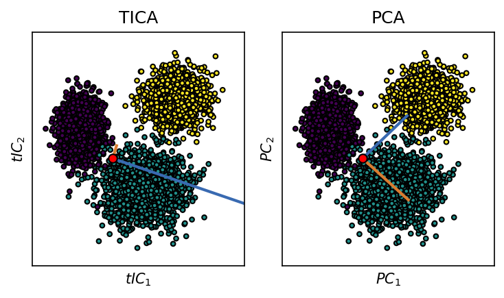
Time-lagged independent component analysis
We want to use TICA as an alternative to PCA to transform the input coordinates into a new set of meaningful coordinates. After TICA, the first obtained coordinate (\(tIC_1\)) is aligned with the axis of slowest geometric change in the input space.
[40]:
system = system_intro
[41]:
# Do TICA
system.tica = pyemma.coordinates.tica(system.traj, var_cutoff=1)
[42]:
# Obtained principle components (n_component, n_dim)
tica_components = system.tica.eigenvectors.T
tica_components
[42]:
array([[ 0.50097289, -0.1844152 ],
       [ 0.01199348,  0.04295948]])
[43]:
# General info
system.tica.describe()
[43]:
'[TICA, lag = 10; max. output dim. = 2]'
[44]:
# Original data projected into TICA-space
projected_trajectory = np.concatenate(system.tica.get_output())
[45]:
# How much information is entailed by the componentes (cummulatively)?
system.tica.cumvar
[45]:
array([0.9921444, 1. ])
[46]:
fig, (tica_ax, pca_ax) = plt.subplots(1, 2)
tica_ax.scatter(
    *system.traj.T,
    c=system.dtraj,
    s=10,
    edgecolors="k", linewidths=1
)

scale = 10
tica_ax.plot([0, tica_components[0, 0] * scale], [0, tica_components[0, 1] * scale], linewidth=2)
tica_ax.plot([0, tica_components[1, 0] * scale], [0, tica_components[1, 1] * scale], linewidth=2)
tica_ax.plot([0], [0], markerfacecolor="red", marker="o", markeredgecolor="k")

pca_ax.scatter(
    *system.traj.T,
    c=system.dtraj,
    s=10,
    edgecolors="k", linewidths=1
)

scale = 2
pca_ax.plot([0, system.pca.components_[0, 0] * scale], [0, system.pca.components_[0, 1] * scale], linewidth=2)
pca_ax.plot([0, system.pca.components_[1, 0] * scale], [0, system.pca.components_[1, 1] * scale], linewidth=2)
pca_ax.plot([0], [0], markerfacecolor="red", marker="o", markeredgecolor="k")

xmin, xmax = system.traj[:, 0].min(), system.traj[:, 0].max()
ymin, ymax = system.traj[:, 1].min(), system.traj[:, 1].max()

limit_factor = 1.2
tica_ax.set(**{
    "xticks": (),
    "yticks": (),
    "xlabel": "$tIC_1$",
    "ylabel": "$tIC_2$",
    "title": "TICA",
    "xlim": (xmin * limit_factor, xmax * limit_factor),
    "ylim": (ymin * limit_factor, ymax * limit_factor),
})

pca_ax.set(**{
    "xticks": (),
    "yticks": (),
    "xlabel": "$PC_1$",
    "ylabel": "$PC_2$",
    "title": "PCA",
    "xlim": (xmin * limit_factor, xmax * limit_factor),
    "ylim": (ymin * limit_factor, ymax * limit_factor),
})

fig.tight_layout()
Exercise
Use pyemma.coordinates.tica to perform a time-lagged independent component analysis on your own data set. Compare the result to the PCA.
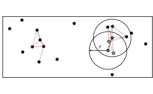
Clustering to generate discrete trajectories
We want to use density-based CommonNN clustering to assign each point in the data set to a (conformational) state.
The algorithm depends on set density criterion:
\(c\) common neighbours with radius \(r\)
[55]:
%%HTML
<video width="90%" src="iteration.mp4" controls></video>
[56]:
system = system_intro
[57]:
# Choose the space
data = np.concatenate(system.tica.get_output())
[58]:
# Prepare for clustering
system.clustering_commonnn = cluster.Clustering(data)
[59]:
# Cluster with given radius and similarity cutoff
system.clustering_commonnn.fit(0.05, 80, member_cutoff=10)
-----------------------------------------------------------------------------------------------
#points   r         c         min       max       #clusters %largest  %noise    time
5000      0.050     80        10        None      3         0.311     0.252     00:00:2.765
-----------------------------------------------------------------------------------------------
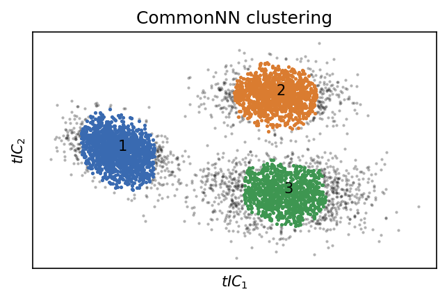
[60]:
fig, ax = plt.subplots()
system.clustering_commonnn.evaluate(ax=ax)
_ = ax.set(**{
    "xticks": (),
    "yticks": (),
    "xlabel": "$tIC_1$",
    "ylabel": "$tIC_2$",
    "title": "CommonNN clustering"
})
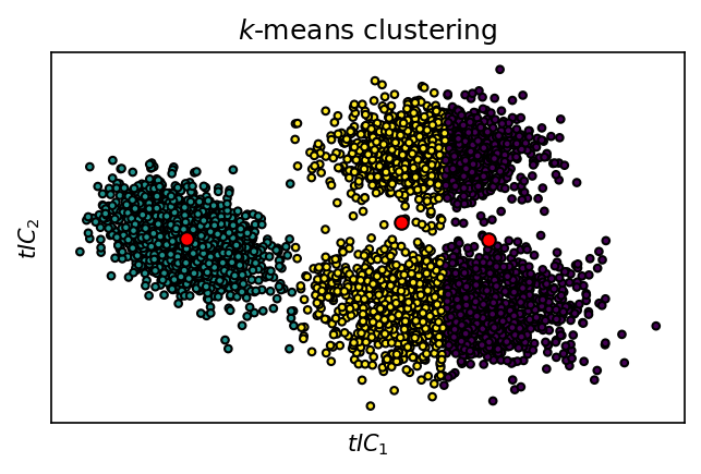
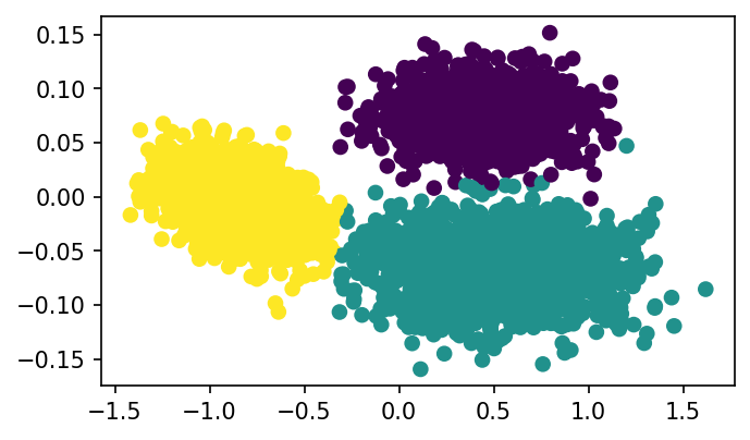
Alternative Voronoi partitioning:
[61]:
system.clustering_voronoi = sklearn.cluster.KMeans(n_clusters=3)
system.clustering_voronoi.fit(data)
[61]:
KMeans(n_clusters=3)
[62]:
fig, ax = plt.subplots()
ax.scatter(
    *data.T,
    c=system.clustering_voronoi.labels_,
    s=10,
    edgecolors="k", linewidths=1
)

ax.plot(*system.clustering_voronoi.cluster_centers_.T, "o", color="red", markeredgecolor="k")

_ = ax.set(**{
    "xticks": (),
    "yticks": (),
    "xlabel": "$tIC_1$",
    "ylabel": "$tIC_2$",
    "title": "$k$-means clustering"
})
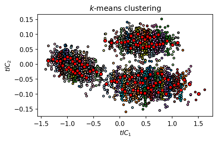
[63]:
system.clustering_voronoi = sklearn.cluster.KMeans(n_clusters=100)
system.clustering_voronoi.fit(data)
[63]:
KMeans(n_clusters=100)
[64]:
fig, ax = plt.subplots()
ax.scatter(
    *data.T,
    c=system.clustering_voronoi.labels_,
    s=10,
    edgecolors="k", linewidths=1,
    cmap=mpl.cm.tab20
)

ax.plot(
    *system.clustering_voronoi.cluster_centers_.T,
    "o",
    color="red",
    markeredgecolor="k",
    markersize=5
)

_ = ax.set(**{
    # "xticks": (),
    # "yticks": (),
    "xlabel": "$tIC_1$",
    "ylabel": "$tIC_2$",
    "title": "$k$-means clustering"
})
Exercise
Take your own data set and subject it to a CommonNN and \(k\)-means clustering.
MSM estimation
Finally, we will try to estimate a transition matrix based on the clustering results.
[74]:
system = system_intro
CommonNN: core set MSM
[75]:
# Expose discrete trajectory
dtrajs = [a - 1 for a in system.clustering_commonnn.to_dtrajs()]
[76]:
dtrajs
[76]:
[array([0, 0, 0, ..., 0, 0, 0])]
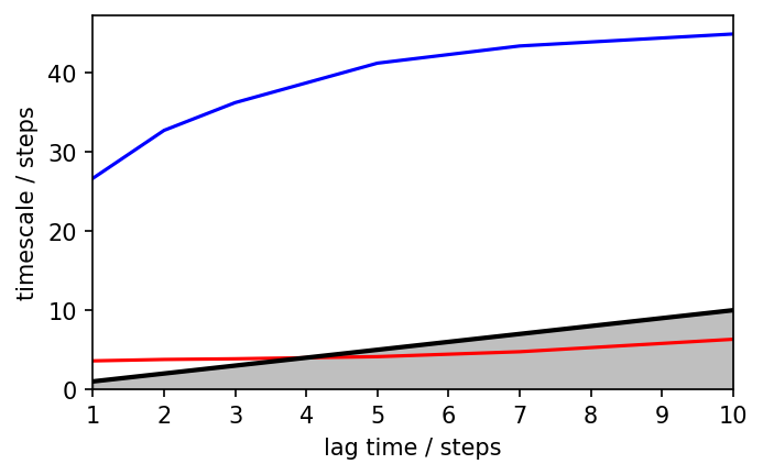
[77]:
# Compute implied timescales for a few different lag times
its = pyemma.msm.its(dtrajs, lags=[1, 2, 3, 5, 7, 10])
08-11-21 15:18:28 pyemma.msm.estimators.maximum_likelihood_msm.MaximumLikelihoodMSM[39] WARNING  Empty core set while unassigned states (-1) in discrete trajectory. Defining core set automatically; check correctness by calling self.core_set.
08-11-21 15:18:28 pyemma.msm.estimators.maximum_likelihood_msm.MaximumLikelihoodMSM[39] WARNING  Empty core set while unassigned states (-1) in discrete trajectory. Defining core set automatically; check correctness by calling self.core_set.
08-11-21 15:18:28 pyemma.msm.estimators.maximum_likelihood_msm.MaximumLikelihoodMSM[39] WARNING  Empty core set while unassigned states (-1) in discrete trajectory. Defining core set automatically; check correctness by calling self.core_set.
08-11-21 15:18:28 pyemma.msm.estimators.maximum_likelihood_msm.MaximumLikelihoodMSM[40] WARNING  Empty core set while unassigned states (-1) in discrete trajectory. Defining core set automatically; check correctness by calling self.core_set.
[78]:
fig, ax = plt.subplots()
pyemma.plots.plot_implied_timescales(its, ylog=False, ax=ax)
ax.set_ylim(0, None)
[78]:
(0.0, 49.293895416904974)
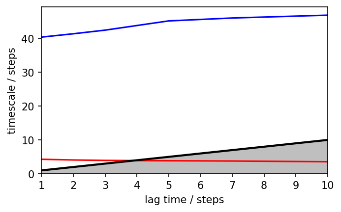
[79]:
# Lag time 2 seems to be reasonable
msm = pyemma.msm.estimate_markov_model(dtrajs, lag=2)
08-11-21 15:18:29 pyemma.msm.estimators.maximum_likelihood_msm.MaximumLikelihoodMSM[39] WARNING Empty core set while unassigned states (-1) in discrete trajectory. Defining core set automatically; check correctness by calling self.core_set.
[80]:
# Transition probability matrix
msm.P
[80]:
array([[0.96853933, 0.02921348, 0.00224719],
       [0.03117506, 0.79076739, 0.17805755],
       [0.00258065, 0.1916129 , 0.80580645]])
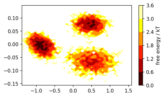
[81]:
# Reweighted free energy surface
fig, ax = plt.subplots()
pyemma.plots.plot_free_energy(
    *system.clustering_commonnn.input_data.T,
    weights=np.concatenate(msm.trajectory_weights()),
    ncontours=5, nbins=50, cmap=mpl.cm.hot,
    ax=ax
)
[81]:
(<Figure size 750x450 with 2 Axes>,
 <matplotlib.axes._subplots.AxesSubplot at 0x7f5159736040>)
[82]:
# Eigenvectors
eigenvectors = msm.eigenvectors_right().T

fig, (ax1, ax2) = plt.subplots(1, 2)
ev = eigenvectors[1]
vmax = np.absolute(ev).max()
ax1.scatter(
    *system.traj.T,
    c=ev[system.dtraj],
    s=10,
    edgecolors="k", linewidths=1,
    cmap=mpl.cm.coolwarm,
    vmin=-vmax, vmax=vmax
)

ev = eigenvectors[2]
vmax = np.absolute(ev).max()
ax2.scatter(
    *system.traj.T,
    c=ev[system.dtraj],
    s=10,
    edgecolors="k", linewidths=1,
    cmap=mpl.cm.coolwarm,
    vmin=-vmax, vmax=vmax
)

for ax in (ax1, ax2):
    ax.set(**{
        "aspect": "equal",
        "xticks": (),
        "yticks": (),
        "xlabel": "$x$",
        "ylabel": "$y$"
    })
k-means: conventional MSM
[83]:
# Expose discrete trajectory
dtrajs = [system.clustering_voronoi.labels_]
[84]:
dtrajs
[84]:
[array([85, 99, 4, ..., 59, 31, 0], dtype=int32)]
[85]:
# Compute implied times scales for a few different lag times
its = pyemma.msm.its(dtrajs, lags=[1, 2, 3, 5, 7, 10], nits=2)
[86]:
fig, ax = plt.subplots()
pyemma.plots.plot_implied_timescales(its, ylog=False, ax=ax)
ax.set_ylim(0, None)
[86]:
(0.0, 47.23439602331783)
[87]:
# Decide for lag time 2
msm = pyemma.msm.estimate_markov_model(dtrajs, lag=2)
[88]:
# Transition probability matrix
msm.P
[88]:
array([[0.04347826, 0.        , 0.        , ..., 0.        , 0.        ,
        0.01429288],
       [0.        , 0.04      , 0.00999952, ..., 0.01999996, 0.01000017,
        0.        ],
       [0.        , 0.00769268, 0.01538462, ..., 0.        , 0.03077123,
        0.        ],
       ...,
       [0.        , 0.03703712, 0.        , ..., 0.03703704, 0.        ,
        0.        ],
       [0.        , 0.00757563, 0.03030106, ..., 0.        , 0.01515152,
        0.        ],
       [0.01206894, 0.        , 0.        , ..., 0.        , 0.        ,
        0.07142857]])
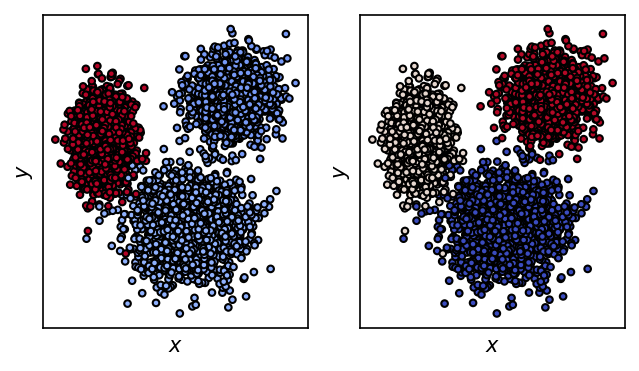
[89]:
# 100 states are hard to interpret. Do PCCA to lump microstates into macrostates.
msm.pcca(3)
[89]:
PCCA(P=array([[0.04348, 0.     , ..., 0.     , 0.01429],
       [0.     , 0.04   , ..., 0.01   , 0.     ],
       ...,
       [0.     , 0.00758, ..., 0.01515, 0.     ],
       [0.01207, 0.     , ..., 0.     , 0.07143]]),
   m=3)
[90]:
# Plot macrostates
msm.metastable_assignments
[90]:
array([2, 1, 0, 1, 2, 0, 1, 0, 2, 2, 1, 1, 1, 0, 1, 2, 1, 1, 2, 1, 0, 1,
       0, 2, 1, 0, 0, 2, 0, 2, 0, 2, 1, 1, 1, 0, 0, 1, 0, 1, 1, 1, 0, 2,
       1, 1, 0, 1, 0, 2, 2, 2, 1, 0, 1, 2, 0, 0, 2, 2, 0, 1, 2, 0, 1, 1,
       2, 2, 1, 2, 1, 0, 2, 0, 2, 1, 2, 2, 1, 0, 0, 0, 1, 2, 0, 2, 0, 1,
       1, 0, 1, 1, 1, 1, 1, 1, 1, 1, 0, 2])
[91]:
fig, ax = plt.subplots()
ax.scatter(
    *system.clustering_commonnn.input_data.T,
    c=msm.metastable_assignments[dtrajs],
)
[91]:
<matplotlib.collections.PathCollection at 0x7f5159c4b310>
Exercise
Estimate a Markov model for your own data set. Plot the original trajectory colored by the right MSM eigenvectors.
Scratch
[104]:
def multivar_gaussian_pdf(x, cov, mu):
    """Multivariate gaussian PDF"""

    n = x.shape[0]

    assert n == mu.shape[0] == cov.shape[0] == cov.shape[1], f"! {n} == {mu.shape[0]} == {cov.shape[0]} == {cov.shape[1]}"

    det = np.linalg.det(cov)
    inv = np.linalg.inv(cov)

    delta_xm = x - mu

    return 1 / ((2 * np.pi)**(n/2) * np.sqrt(det)) * np.exp(-0.5 * (delta_xm.T @ inv @ delta_xm))