![]()
AlgoSB 2021
Practical afternoon session Monday, 8th of November. VGLAPG example trajectory analysis.
[1]:
import sys
import warnings

import cnnclustering
from cnnclustering import cluster, hooks, plot
from IPython.core.display import display, HTML
import matplotlib as mpl
import matplotlib.pyplot as plt
import mdtraj as md
import nglview as nv
import numpy as np
import pyemma
import scipy
import scipy.linalg
import sklearn
from sklearn.metrics import pairwise_distances
from sklearn.neighbors import KDTree
Uncomment and execute the following lines of code if you are on Google Colab to make nglview work:
[2]:
# from google.colab import output
# output.enable_custom_widget_manager()
[3]:
# Jupyter display settings
display(HTML("<style>.container { width:90% !important; }</style>"))
[4]:
# Version information
print("Python: ", *sys.version.split("\n"))

print("Packages:")
for package in [mpl, np, scipy, sklearn, pyemma, cnnclustering, nv]:
    print(f"    {package.__name__}: {package.__version__}")
Python:  3.8.12 | packaged by conda-forge | (default, Oct 12 2021, 21:59:51)  [GCC 9.4.0]
Packages:
    matplotlib: 3.4.3
    numpy: 1.21.4
    scipy: 1.7.2
    sklearn: 1.0.1
    pyemma: 2.5.9
    cnnclustering: 0.5.0
    nglview: 3.0.3
[5]:
mpl.rc_file('../matplotlibrc')
[6]:
warnings.simplefilter("ignore")
Load data
We will work here with a 600 ns trajectory of the hexapeptide VGLAPG. We want to analyze the dynamics of its backbone and therefore use the backbone phi/psi dihedrals as our features of interest. The provided trajectory is a NumPy array of shape (600001, 10). The first 5 columns are the phi dihedrals, the last 5 columns are the psi dihedrals. The timestep of the trajectory is 1 ps.
[7]:
t_1ns = md.load('traj_dt_1ns.xtc', top='VGLAPG.pdb')
mview = nv.show_mdtraj(t_1ns)
mview.add_licorice()
mview
[8]:
dihed_traj = np.load('VGLAPG_dihedrals.npy')
res_names = ['VAL1', 'GLY2', 'LEU3', 'ALA4', 'PRO5', 'GLY6']
[9]:
dihed_traj.shape
[9]:
(600001, 10)
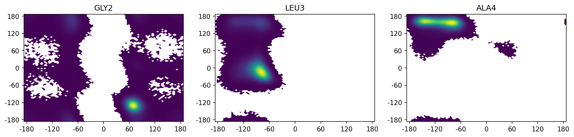
We plot the ramachandran plots for the inner three aminoacids. Note that the ramachandran plot for the terminal aminoacids is not possible as the N-terminal aminoacid does not have a psi dihedral and the C-terminal aminoacid does not have a phi dihedral.
[10]:
fig, axs = plt.subplots(1, 3, figsize=(15, 3))
for i in range(1, 4):
    ax = axs[i - 1]
    pyemma.plots.plot_density(dihed_traj[:, i - 1], dihed_traj[:, i + 5], ax=ax, cbar=False)
    axs[i - 1].set_title(res_names[i])

    ax.set_xticks(np.arange(-3, 3.1, 1))
    ax.set_xticklabels(np.arange(-180, 181, 60))
    ax.set_yticks(np.arange(-3, 3.1, 1))
    ax.set_yticklabels(np.arange(-180, 181, 60))
TICA
We want to reduce our 10 dimensional data to 2 dimensions, which are easy to plot and a much simpler system. As we are not interested in rapidly changing dynamics and want to have a look at the slow dynamic processes of the backbone, we choose time-lagged independent component analysis (TICA) as our method of coordinate transformation.
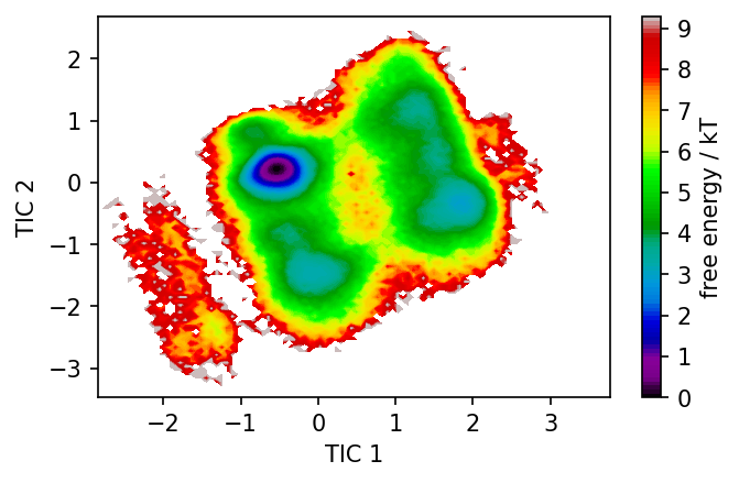
Exercise
Reduce the 10-dimensional trajectory data to 2 TIC dimensions using the PyEmma TICA module. Plot the density or free energy of the trajectory data in the space of the TIC dimensions.
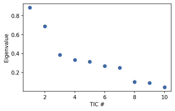
[11]:
tica = pyemma.coordinates.tica(dihed_traj, dim=2)
[12]:
fig, ax = plt.subplots()
ax.plot(np.arange(1, 11, 1), tica.eigenvalues, 'o')
ax.set_ylabel('Eigenvalue')
ax.set_xlabel('TIC #')
[12]:
Text(0.5, 0, 'TIC #')
[13]:
fig, ax = plt.subplots()
pyemma.plots.plot_free_energy(np.concatenate(tica.get_output())[:, 0], np.concatenate(tica.get_output())[:, 1], ax=ax)
ax.set_xlabel('TIC 1')
ax.set_ylabel('TIC 2')
[13]:
Text(0, 0.5, 'TIC 2')
CommonNN Clustering
We want to create a Markov State Model on the 2D TICA data to study slow processes of the backbone dynamics. In the first step we need to discretize the 2D TICA space with a clustering method. Core-set MSMs based on density based clustering have proven to show good convergence, even with large biosystems, so we apply th density based CommonNN clustering algorithm. As the cluster fitting can get time-intensive for large datasets, we here reduce the dataset size by taking only every tenth point into account. This raises the timestep to 10 ps.
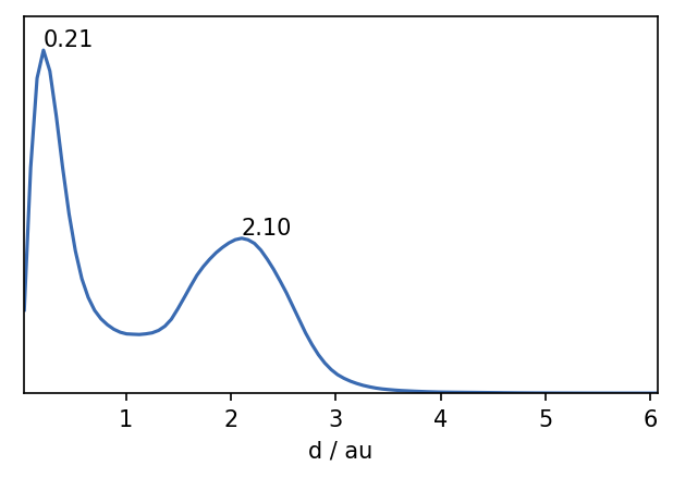
For CommonNN clustering we need to define the three parameters radius, neighbor cutoff and member cutoff. It is usually advisable to plot the pairwise distances of the dataset and choose a radius slightly shorter than the first maximum. We chose a radius of 0.2, a neighbor cutoff of 500 and a member cutoff of 10.
[14]:
data = np.concatenate(tica.get_output())[::10]
[15]:
distances = pairwise_distances(data[::10])
distance_rclustering = cluster.Clustering(distances, registered_recipe_key="distances")

fig, ax = plt.subplots()
_ = plot.plot_histogram(ax, distances.flatten(), maxima=True, maxima_props={"order": 5})
Clustering can be memory intensive. If you run this notebook and do not have the necessary memory available, you can load the pre-calculated labels.
[16]:
clustering = cluster.Clustering(data)

# Pre-compute and sort neighbourhoods and choose the corresponding recipe
tree = KDTree(data)
neighbourhoods = tree.query_radius(
    data, r=0.2, return_distance=False
    )

for n in neighbourhoods:
    n.sort()

# Custom initialisation using a clustering builder
clustering_neighbourhoods_sorted = cluster.Clustering(
    neighbourhoods,
    preparation_hook=hooks.prepare_neighbourhoods,
    registered_recipe_key="sorted_neighbourhoods"
    )
[17]:
# Use pre-computed neighbourhoods
clustering_neighbourhoods_sorted.fit(0.2, 550, 10)
clustering._labels = clustering_neighbourhoods_sorted._labels
-----------------------------------------------------------------------------------------------
#points   r         c         min       max       #clusters %largest  %noise    time
60001     0.200     550       10        None      3         0.587     0.231     00:00:14.218
-----------------------------------------------------------------------------------------------
[18]:
# To load provided labels (in case of insufficient memory):
clustering = cluster.Clustering(data)
clustering.labels = np.load('cluster_labels.npy')
[19]:
_ = clustering.evaluate()
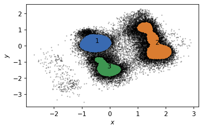
We identified 3 clusters that we can plot in TICA space. Points outside the clusters are considered as noise.
Visualization
[20]:
t_cluster_centers = md.load('t_cluster_centers.xtc', top='VGLAPG.pdb')
[21]:
mview = nv.show_mdtraj(t_cluster_centers)
mview.add_licorice()
mview
Markov State Model
To build the MSM we apply the PyEMMA package. Firstly, we have to adjust our discretized trajectories from the clustering, because noise in CNN clustering is indicated by the cluster number 0, while in PyEMMA it is -1. We adjust the dataset by substracting 1 from every cluster number.
[22]:
dtrajs = [x - 1 for x in clustering.to_dtrajs()]
Exercise
Build a Markov Sate Model using the PyEMMA package and the discretized trajectory from the clustering. Create an implied timescales plot to choose an appropriate lag-time. Plot the first two left and right eigenvectors.
[23]:
its = pyemma.msm.its(dtrajs, lags=[1, 2, 5, 10, 20, 50, 100, 200], nits=3)
pyemma.plots.plot_implied_timescales(its, ylog=False, dt=0.01, units='ns')
05-11-21 17:53:49 pyemma.msm.estimators.maximum_likelihood_msm.MaximumLikelihoodMSM[5] WARNING  Empty core set while unassigned states (-1) in discrete trajectory. Defining core set automatically; check correctness by calling self.core_set.
05-11-21 17:53:49 pyemma.msm.estimators.maximum_likelihood_msm.MaximumLikelihoodMSM[5] WARNING  Empty core set while unassigned states (-1) in discrete trajectory. Defining core set automatically; check correctness by calling self.core_set.
05-11-21 17:53:49 pyemma.msm.estimators.maximum_likelihood_msm.MaximumLikelihoodMSM[5] WARNING  Empty core set while unassigned states (-1) in discrete trajectory. Defining core set automatically; check correctness by calling self.core_set.
05-11-21 17:53:49 pyemma.msm.estimators.maximum_likelihood_msm.MaximumLikelihoodMSM[5] WARNING  Empty core set while unassigned states (-1) in discrete trajectory. Defining core set automatically; check correctness by calling self.core_set.
05-11-21 17:53:49 pyemma.msm.estimators.maximum_likelihood_msm.MaximumLikelihoodMSM[5] WARNING  Empty core set while unassigned states (-1) in discrete trajectory. Defining core set automatically; check correctness by calling self.core_set.
05-11-21 17:53:49 pyemma.msm.estimators.maximum_likelihood_msm.MaximumLikelihoodMSM[5] WARNING  Empty core set while unassigned states (-1) in discrete trajectory. Defining core set automatically; check correctness by calling self.core_set.
05-11-21 17:53:49 pyemma.msm.estimators.maximum_likelihood_msm.MaximumLikelihoodMSM[6] WARNING  Empty core set while unassigned states (-1) in discrete trajectory. Defining core set automatically; check correctness by calling self.core_set.
05-11-21 17:53:49 pyemma.msm.estimators.maximum_likelihood_msm.MaximumLikelihoodMSM[6] WARNING  Empty core set while unassigned states (-1) in discrete trajectory. Defining core set automatically; check correctness by calling self.core_set.
05-11-21 17:53:50 pyemma.msm.estimators.implied_timescales.ImpliedTimescales[3] WARNING  Changed user setting nits to the number of available timescales nits=2
[23]:
<matplotlib.axes._subplots.AxesSubplot at 0x7f4e7b5eafd0>
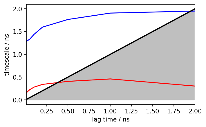
We see the implied timescales converge at a lag time of about 1 ns, which we take as the lagtime for our MSM.
[24]:
MSM = pyemma.msm.estimate_markov_model(dtrajs, lag=100)
05-11-21 17:53:50 pyemma.msm.estimators.maximum_likelihood_msm.MaximumLikelihoodMSM[5] WARNING Empty core set while unassigned states (-1) in discrete trajectory. Defining core set automatically; check correctness by calling self.core_set.
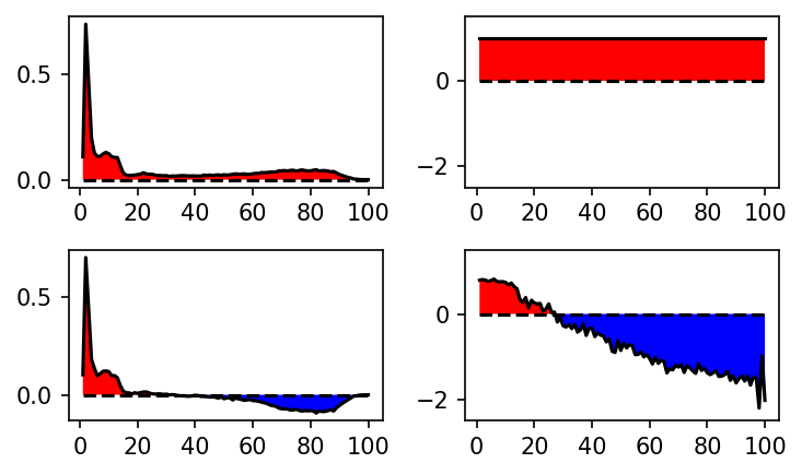
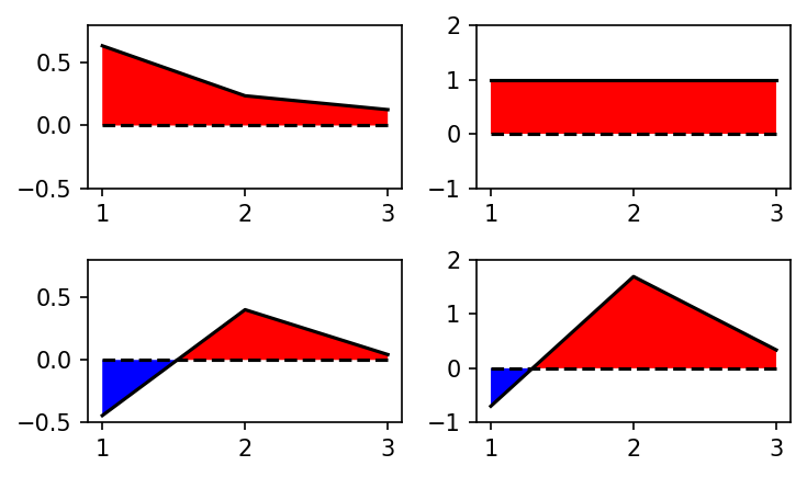
We can analyze the MSM by plotting its eigenvectors.
[25]:
def plot_eigenvector(ax, eig):
    '''Plot eigenvector.'''
    x = np.arange(1, len(eig) + 1, 1)
    y = eig
    ax.plot(x, y, color='k')
    ax.plot(x, [0]*len(x), '--', color='k')
    ax.fill_between(x, 0, y, where= y>=0, facecolor='red', interpolate=True)
    ax.fill_between(x, 0, y, where= y<=0, facecolor='blue', interpolate=True)

fig, axs = plt.subplots(2, 2)
plot_eigenvector(axs[0][0], MSM.eigenvectors_left()[0])
plot_eigenvector(axs[1][0], MSM.eigenvectors_left()[1])
plot_eigenvector(axs[0][1], MSM.eigenvectors_right()[:, 0])
plot_eigenvector(axs[1][1], MSM.eigenvectors_right()[:, 1])

for ax in axs[:, 0]:
    ax.set_ylim(-0.5, 0.8)
for ax in axs[:, 1]:
    ax.set_ylim(-1, 2)

for ax in axs.flat:
    ax.set_xticks(np.arange(1, 4, 1))
plt.tight_layout()
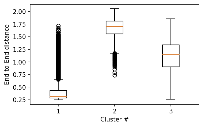
Open-Close Transition
[26]:
d_ete_traj = np.load('VGLAPG_end_to_end.npy')
[27]:
ete_data = []
for i in range(1, 4):
    x = d_ete_traj[np.where(clustering.to_dtrajs()[0] == i, True, False)]
    ete_data.append(x)
[28]:
fig, ax = plt.subplots()
ax.boxplot(ete_data)
ax.set_ylabel('End-to-End distance')
ax.set_xlabel('Cluster #')
plt.show()
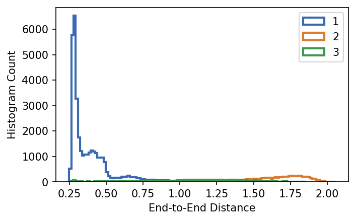
Exercise
Plot the distribution of the end-to-end distance within the clusters as histograms.
[29]:
fig, ax = plt.subplots()
ax.hist(ete_data[0], histtype='step', linewidth=2, bins=100, label='1')
ax.hist(ete_data[1], histtype='step', linewidth=2, bins=100, label='2')
ax.hist(ete_data[2], histtype='step', linewidth=2, bins=100, label='3')
ax.set_xlabel('End-to-End Distance')
ax.set_ylabel('Histogram Count')
plt.legend()
plt.show()
Markov State Model on End-to-End Distance
While we use packages like PyEmma to create MSMs, it is also possible to code them manually, and for a simple case like a 1D MSM quite straightforward. Here we show how to create an MSM using only python and numpy. We use the end-to-end distance of VGLAPG as our coordinate.
[30]:
# Load End-to-End Distance Data
d = d_ete_traj

# Get Range For Discretization
d_min = np.amin(d)
d_max = np.amax(d) + 0.01
d_range = d_max - d_min

# Set How Many States for Discretization
n_states = 100
delta_d = d_range / n_states

# Discretize Trajectory
d_discretized = np.floor((d - d_min) / delta_d).astype('int')
d_discretized = d_discretized

# Initialize Count Matrix and Set Lag-Time tau
C = np.zeros((n_states,n_states))
tau = 100

# Count State Transtitions and Store in Count Matrix
for x in range(len(d_discretized) - tau):
    state_i = d_discretized[x]
    state_j = d_discretized[x + tau]
    C[state_i, state_j] += 1

# Enforce Detailed Balance
C_db = C + np.transpose(C)

# Create Transition Matrix By Row-Normalizing Count Matrix
T = np.zeros((n_states, n_states))
for i in range(n_states):
    T[i, :] = C[i, :] / np.sum(C[i, :])

# Calculate Left and Right Eigenvectors
eig_right = np.real(np.linalg.eig(T)[1])
eig_left = np.real(np.linalg.eig(T.T)[1])
[31]:
fig, axs = plt.subplots(2, 2)
plot_eigenvector(axs[0][0], eig_left[:, 0])
plot_eigenvector(axs[1][0], eig_left[:, 1] * -1)
plot_eigenvector(axs[0][1], eig_right[:, 0] * 10)
plot_eigenvector(axs[1][1], eig_right[:, 1] * -10)

for ax in axs[:, 1]:
    ax.set_ylim(-2.5, 1.5)

for ax in axs.flat:
    ax.set_xticks(np.arange(0, 101, 20))
plt.tight_layout()