Introduction to Molecular Dynamics simulations with OpenMM
Running Molecular Dynamics (MD) simulations of all possible kinds of molecular systems in a correct and efficient way is a non-trivial task. Luckily, there are many different programs and packages out there to help you with that. Due to the complexity of the matter, however, these programs are mostly not exactly straightforward to use. All of them have their strengths and weaknesses and come with their own flavor of addressing the exercise of representing molecules in silico and propagating their configuration through time. The basic concepts underlying their design are often very similar, though. We chose the open source toolkit OpenMM to practically introduce you to the art of molecular simulations, because it provides a relatively well accessible interface in Python. Although it is not as feature rich out of the box as other solutions, it is successfully used in daily research.
We will show you here step-by-step how to setup and run a standard NVT MD simulation of a protein in water with OpenMM. Refer to the official website for installation instructions (OpenMM is available in the conda package manager) and documentation. We will also need some kind of molecule viewer to inspect molecular structures. We can recommend VMD for this purpose (also available via conda).
conda install -c omnia -c conda-forge openmm
conda install -c conda-forge vmd
To completely follow this introduction, you will also need the PDBFixer that has to be installed separately. You will not need the PDBFixer for the upcoming exercise.
$ git clone https://github.com/openmm/pdbfixer.git
$ cd pdbfixer
$ python setup.py install
Pre-requirements
[1]:
import shlex       # Optional
import subprocess  # Optional

import matplotlib as mpl
import matplotlib.pyplot as plt
[2]:
# Matplotlib configuration
mpl.rcParams.update(mpl.rcParamsDefault)
mpl.rc_file('../../matplotlibrc', use_default_template=False)
Primer on molecular structure files
A central element of every molecular simulation is the (atomic) structure of the system of interest. In a classic MD simulation every atom in the system is represented as a point in \(\mathbb{R}^3\) with \(x\)-, \(y\)-, and \(z\)-coordinates. We need to provide these coordinates in a machine (and human) readable, consistent format to be of any use in a computer simulation. A popular file format, especially for biochemical systems, is the PDB file format. PDB files (filename extension .pdb) are text files and can be opened with the text editor of your choice. Many (crystal-, NMR-, cryoEM-, …) structures that can be used as starting structures in simulations are available in the RCSB Protein Data Bank (PDB) for everyone to download. Structures in this data base are identified by a letter code – the PDB-ID. For our example, we use the Structure of the carbohydrate-recognition domain of human Langerin with the PDB-ID 3P5G. Langerin is an endocytic pattern recognition receptor important for the human immune system.
Info: If you want to learn more about PDB structure files than we tackle here, check out this Guide to understanding PDB data.
[3]:
# Lets have a look into the PDB file
with open("3p5g.pdb") as pdb_file:
    show = 10  # Lines to show
    for lc, line in enumerate(pdb_file):
        # Print the first lines of the file
        if lc < show:
            print(line.strip())
print("=" * 80)
print("Total line count: ", lc)
HEADER    SUGAR BINDING PROTEIN                   08-OCT-10   3P5G
TITLE     STRUCTURE OF THE CARBOHYDRATE-RECOGNITION DOMAIN OF HUMAN LANGERIN
TITLE    2 WITH BLOOD GROUP B TRISACCHARIDE (GAL ALPHA1-3(FUC ALPHA1-2)GAL)
COMPND    MOL_ID: 1;
COMPND   2 MOLECULE: C-TYPE LECTIN DOMAIN FAMILY 4 MEMBER K;
COMPND   3 CHAIN: A, B, C, D;
COMPND   4 FRAGMENT: LANGERIN CRD (UNP RESIDUES 193-328);
COMPND   5 SYNONYM: LANGERIN;
COMPND   6 ENGINEERED: YES
SOURCE    MOL_ID: 1;
================================================================================
Total line count:  5922
Each line in the PDB file begins with a record keyword identifying the kind of information stored in the corresponding line. Records like HEADER, TITLE, or COMPND contain information that we can safely ignore when we are only interested in the atomic coordinates of the molecule. Depending on what you want to find out about the structure, however, they can be very useful. The COMPND statements tells us for example, that the file contains 4 (identical) subunits – so called chains
A, B, C, and D – each consisting of 136 amino acid residues (residues 193 to 328). We can also get the complete sequence of the protein contained in this file from SEQRES entries.
[4]:
# What is the protein sequence?
with open("3p5g.pdb") as pdb_file:
    for line in pdb_file:
        if line.startswith("SEQRES"):
            line = line.split()
            if line[2] == "A":
                # Only print sequence for chain A
                print(*line[4:])
GLN VAL VAL SER GLN GLY TRP LYS TYR PHE LYS GLY ASN
PHE TYR TYR PHE SER LEU ILE PRO LYS THR TRP TYR SER
ALA GLU GLN PHE CYS VAL SER ARG ASN SER HIS LEU THR
SER VAL THR SER GLU SER GLU GLN GLU PHE LEU TYR LYS
THR ALA GLY GLY LEU ILE TYR TRP ILE GLY LEU THR LYS
ALA GLY MET GLU GLY ASP TRP SER TRP VAL ASP ASP THR
PRO PHE ASN LYS VAL GLN SER ALA ARG PHE TRP ILE PRO
GLY GLU PRO ASN ASN ALA GLY ASN ASN GLU HIS CYS GLY
ASN ILE LYS ALA PRO SER LEU GLN ALA TRP ASN ASP ALA
PRO CYS ASP LYS THR PHE LEU PHE ILE CYS LYS ARG PRO
TYR VAL PRO SER GLU PRO
Often a PDB file contains more than only the structure of the main molecule. Crystallographic structures for example can contain co-crystallised solvent and salt as well as ligands like small drug like molecules. Record entries like HETNAM or FORMULA may tell you more about what else is in your file. Our example comes with a sugar ligand, a calcium-ion, and crystal water.
[5]:
# What else is in the file?
with open("3p5g.pdb") as pdb_file:
    for line in pdb_file:
        if line.startswith(("HETNAM", "FORMUL")):
            print(line.strip())
HETNAM     GLA ALPHA D-GALACTOSE
HETNAM     GAL BETA-D-GALACTOSE
HETNAM     FUC ALPHA-L-FUCOSE
HETNAM      CA CALCIUM ION
FORMUL   5  GLA    3(C6 H12 O6)
FORMUL   5  GAL    C6 H12 O6
FORMUL   5  FUC    4(C6 H12 O5)
FORMUL   6   CA    4(CA 2+)
FORMUL  13  HOH   *816(H2 O)
Finally, the atomic coordinates we were initially interested in are listed under ATOM records. From left to right, each ATOM record holds the atom ID, atom name, residue name, chain ID, residue ID, xyz-coordinates in Å, crystallographic occupancy, crystallographic temperature factor and the chemical element of a single atom in a strict order. The different parts are identify by a character position, i.e. the chain ID for example occupies the 22nd character of the
ATOM entry. Besides the xyz-coordinates, for an MD simulation we need especially the atom name and the residue name column. To represent an atom in such a simulation by suitable force field parameters, it is not enough to know that we have for example a carbon atom somewhere. It is required to know instead that it is say the C\(_\mathsf{α}\)-atom of a glycine. Note, that the first residue in chain A is GLY198 which means that residues 193 to 197 are missing in this chain.
[6]:
with open("3p5g.pdb") as pdb_file:
    show = 10
    count = 0
    # Print the first ATOM entries
    for line in pdb_file:
        if count >= show:
            break
        if line.startswith(("ATOM")):
            print(line.strip())
            count += 1
ATOM      1  N   GLY A 198       1.923  33.617   6.889  1.00 29.44           N
ATOM      2  CA  GLY A 198       2.927  34.067   5.942  1.00 33.42           C
ATOM      3  C   GLY A 198       4.064  33.079   5.747  1.00 21.30           C
ATOM      4  O   GLY A 198       5.016  33.355   5.022  1.00 26.76           O
ATOM      5  N   TRP A 199       3.964  31.919   6.391  1.00 19.08           N
ATOM      6  CA  TRP A 199       4.990  30.892   6.261  1.00 19.93           C
ATOM      7  C   TRP A 199       4.987  30.356   4.840  1.00 28.23           C
ATOM      8  O   TRP A 199       3.926  30.117   4.255  1.00 30.68           O
ATOM      9  CB  TRP A 199       4.772  29.756   7.263  1.00 22.11           C
ATOM     10  CG  TRP A 199       4.961  30.161   8.697  1.00 19.73           C
Atoms not part of the main molecule are usually put into HETATM records of similar structure. TER additionally marks the end of a chain, which is particularly important for proteins because the termini are modeled differently than residues within the chain.
[7]:
with open("3p5g.pdb") as pdb_file:
    show = 34
    count = 0
    # Print the first HETATM entries
    for line in pdb_file:
        if count >= show:
            break
        if line.startswith(("HETATM")):
            print(line.strip())
            count += 1
HETATM 4215  C1  GLA A 400      35.389  42.564   1.554  1.00 34.53           C
HETATM 4216  C2  GLA A 400      34.417  41.967   0.543  1.00 38.46           C
HETATM 4217  C3  GLA A 400      33.765  40.724   1.124  1.00 24.16           C
HETATM 4218  C4  GLA A 400      34.841  39.740   1.563  1.00 25.80           C
HETATM 4219  C5  GLA A 400      35.798  40.434   2.520  1.00 33.42           C
HETATM 4220  C6  GLA A 400      36.930  39.510   2.960  1.00 35.43           C
HETATM 4221  O2  GLA A 400      33.406  42.903   0.245  1.00 35.44           O
HETATM 4222  O3  GLA A 400      32.945  40.132   0.148  1.00 34.77           O
HETATM 4223  O4  GLA A 400      35.543  39.288   0.424  1.00 26.84           O
HETATM 4224  O5  GLA A 400      36.347  41.582   1.899  1.00 48.07           O
HETATM 4225  O6  GLA A 400      37.680  40.140   3.977  1.00 26.17           O
HETATM 4226  C1  GAL A 401      35.691  44.693   5.881  1.00 58.00           C
HETATM 4227  C2  GAL A 401      34.721  44.101   4.866  1.00 34.37           C
HETATM 4228  C3  GAL A 401      35.517  43.473   3.723  1.00 26.42           C
HETATM 4229  C4  GAL A 401      36.531  44.479   3.176  1.00 47.76           C
HETATM 4230  C5  GAL A 401      37.356  45.105   4.295  1.00 46.54           C
HETATM 4231  C6  GAL A 401      38.282  46.188   3.748  1.00 66.04           C
HETATM 4232  O1  GAL A 401      34.968  45.256   6.951  1.00 41.39           O
HETATM 4233  O2  GAL A 401      33.927  43.149   5.553  1.00 30.54           O
HETATM 4234  O3  GAL A 401      34.648  43.055   2.689  1.00 32.94           O
HETATM 4235  O4  GAL A 401      35.864  45.510   2.481  1.00 33.15           O
HETATM 4236  O5  GAL A 401      36.495  45.674   5.258  1.00 38.71           O
HETATM 4237  O6  GAL A 401      38.986  46.792   4.811  1.00 54.30           O
HETATM 4238  C1  FUC A 402      32.629  42.960   4.961  1.00 22.64           C
HETATM 4239  C2  FUC A 402      31.943  41.857   5.765  1.00 19.14           C
HETATM 4240  C3  FUC A 402      31.667  42.330   7.178  1.00 15.88           C
HETATM 4241  C4  FUC A 402      30.867  43.622   7.148  1.00 22.27           C
HETATM 4242  C5  FUC A 402      31.577  44.638   6.258  1.00 18.90           C
HETATM 4243  C6  FUC A 402      30.712  45.886   6.131  1.00 32.10           C
HETATM 4244  O2  FUC A 402      32.798  40.739   5.847  1.00 24.94           O
HETATM 4245  O3  FUC A 402      30.972  41.311   7.888  1.00 20.82           O
HETATM 4246  O4  FUC A 402      29.573  43.399   6.633  1.00 25.32           O
HETATM 4247  O5  FUC A 402      31.822  44.121   4.962  1.00 24.17           O
HETATM 4248 CA    CA A 500      32.105  39.059   7.647  1.00 19.65          CA
To get a better overview over the system, let’s open the PDB file in VMD (start VMD directly from the Jupyter notebook for a quick view or externally otherwise).
[8]:
# Lauch VMD from Jupyter
view = subprocess.Popen(
    shlex.split("vmd 3p5g.pdb"),
    close_fds=True,
    stdin=subprocess.PIPE,
    stdout=subprocess.PIPE,
    stderr=subprocess.PIPE
)
We display the protein chains in the NewCartoon representation, colored by SecondaryStructure. For the Ca-ion we use the VDW representation and color it with a ColorID of our choice. Water and ligand atoms are shown in the Licorice representation and colored by Name. You can set these options in the Main > Graphics > Representations... menu. Note, that the structure does not contain hydrogen atoms.
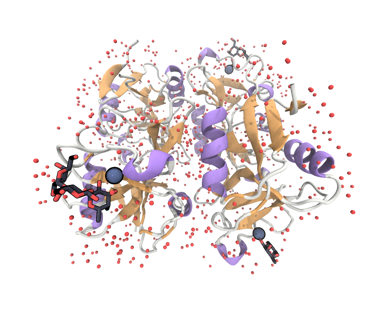
FIGURE Full structure under the PDB entry 3P5G, showing 4 langerin molecules with calcium atoms, crystal water and different sugar ligands bound.
Fixing and modifying the structure
For our simulation we now want to extract only chain A including the present protein residues 198 to 325. You could do this in VMD via Main > File > Save Coordinates... but meta information stored in the file is usually lost this way. You can perform this task manually by just deleting information you do not need from the text file. The best way in terms of reproducibility and traceability, however, might be to use Python for this. Note, that we have to issues to deal with here:
We need to pay separate attention in our case to residues that have atom entries with split occupancies, a leftover of the crystal structure prediction, like for SER277 shown below. For this residue two alternative sets of atoms are given, indicated by a letter at the 17th character of the
ATOMentry.We want to reconstruct the missing residues 193 to 197 and 326 to 328. In particular we want to fix missing terminal atoms in this way.
[9]:
# Check structure for alternative atom positions
with open("3p5g.pdb") as pdb_file:
    for line in pdb_file:
        if not line.startswith("ATOM"):
            continue
        if not line[21] == "A":  # Chain A?
            continue
        if line[16] != " ":      # Alternativ atoms positions?
            print(line.strip())
ATOM    658  CA ASER A 277      29.047  24.388   2.751  0.50 19.39           C
ATOM    659  CA BSER A 277      29.040  24.387   2.738  0.50 18.11           C
ATOM    662  CB ASER A 277      28.811  24.669   4.239  0.50 18.59           C
ATOM    663  CB BSER A 277      28.762  24.666   4.218  0.50 17.85           C
ATOM    664  OG ASER A 277      27.712  23.928   4.738  0.50 15.78           O
ATOM    665  OG BSER A 277      29.938  24.530   4.996  0.50 17.39           O
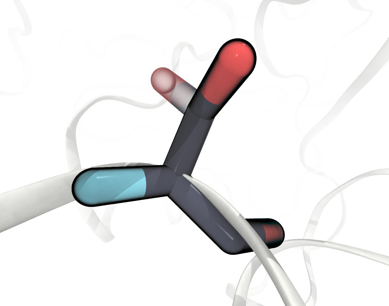
FIGURE SER277 has two alternative sets of atom positions in the PDB File, one displayed transparentl
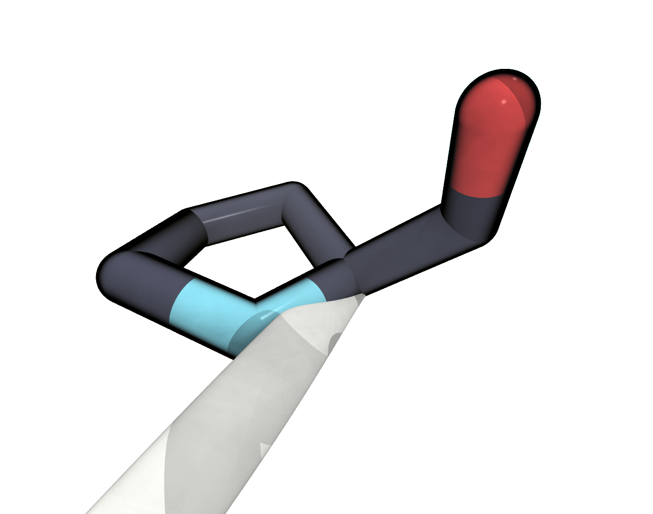
FIGURE The terminal PRO325 is missing a terminal oxygen atom.
Let’s tackle the ambiguous atom positions first. We can fix this kind of shortcoming easily while extracting atom information from the file.
[10]:
allowed_res_ids = list(range(198, 326)) + [500]
# Protein 198 to 325 and Ca

# Copy desired information from one file to another
with open("3p5g.pdb") as in_file:
    with open("chain_A.pdb", "w") as out_file:
        for line in in_file:
            if line.startswith(("ATOM", "TER", "HETATM")):
                # check for atomic entries
                if not line[21] == "A":
                    # Chain A?
                    continue
                if not int(line[22:26]) in allowed_res_ids:
                    # Keep residue?
                    continue
                if line[16] == "B":  # Alternative set of atoms?
                    # Throw away location B
                    continue
                if line[16] == "A":  # Alternative set of atoms?
                    # Keep location A
                    line = line[:16] + " " + line[17:]
            out_file.write(line)
The second task, adding missing residues and atoms, can not be so easily solved by ourselves. We will use a tool from the OpenMM cosmos for this – the PDBFixer. This tool can be used through a Python interface. To save the fixed PDB file back to disk we will also need the PDB file handler from the OpenMM package. We will discuss the file handling by OpenMM more in the next section.
[11]:
import pdbfixer
import simtk.openmm.app as app  # OpenMM interface
The fixing work the following way: We create a PDBFixes Python object from our pre-processed PDB file. Than we let the fixer find missing residues, which it does by analysing the header of the PDB file (which is why we wanted to let it be in there). Finally we can fix the missing atoms and save to a new PDB file.
[12]:
fixer = pdbfixer.PDBFixer("chain_A.pdb")  # Load file
fixer.findMissingResidues()               # Identify missing residues
fixer.findMissingAtoms()                  # Identify missing atoms
print(fixer.missingResidues)
{(0, 0): ['GLN', 'VAL', 'VAL', 'SER', 'GLN'], (0, 128): ['SER', 'GLU', 'PRO']}
The PDBFixer found, that in chain A (0) at the beginning (residue id 0) five residues, and at the end (residue id 128) three residues should be added. The fixer.missingResidues attribute tells us this in form of a Python dictionary having tuples of (chain ID, residue ID) has keys (points to insert residues) and lists of residues as values. We are fine with that and proceed with applying the changes.
[13]:
fixer.addMissingAtoms()  # Apply the fix
app.PDBFile.writeFile(fixer.topology, fixer.positions, open('chain_A_fixed.pdb', 'w'))
# Save to file
There is one last thing we want to repair. The PDBFixer renumbered the residues in the protein from 1 to 136 and we would like to restore the biological numbering starting at 193 going to 328. Note also, that the PDBFixer put the calcium atom in a another chain B than the protein and omitted the PDB meta-information, but we are fine with that at this point.
[14]:
offset = 192 # Residue numbering should start here

# Fix residue numbering
with open('chain_A_fixed.pdb') as in_file:
    with open('chain_A_fixednumbering.pdb', "w") as out_file:
        for line in in_file:
            if line.startswith(("ATOM", "TER", "HETATM")) and line[21] == "A":
                resid = int(line[22:26]) + offset
                line = line[:22] + f"{resid:>4}" + line[26:]
            out_file.write(line)
We visualise the reduced and fixed structure – now only containing a single langerin chain plus calcium atom – once more in VMD, this time using the QuickSurf representation and coloring by Name. In the next part we will prepare this structure for a standard simulation in water.
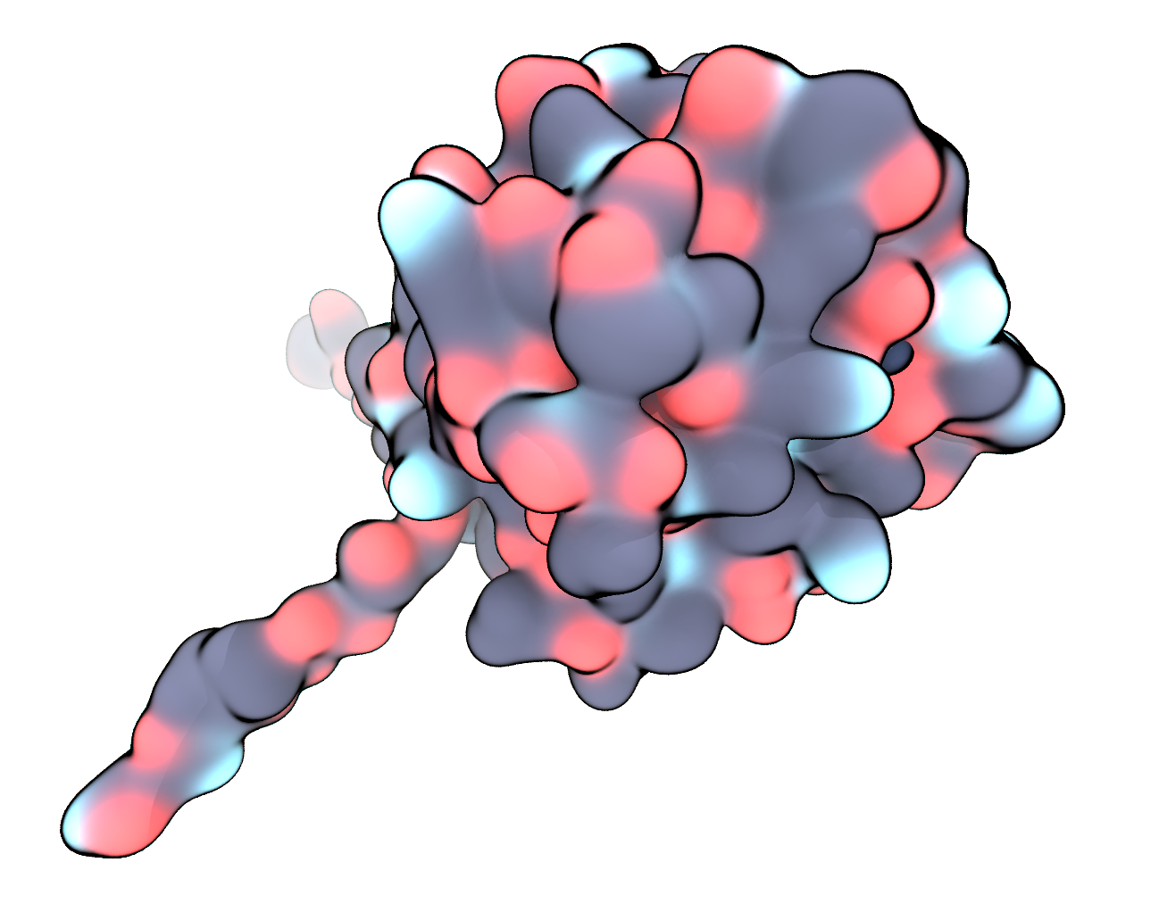
FIGURE Pre-processed langerin structure in surface representation, carbon – black, oxygen – red, nitrogen – blue, sulfur – yellow, calcium – dark blue.
Structure preparation with OpenMM
To use OpenMM to prepare our structure further for the simulation in water we need to import a few Python modules.
[15]:
import simtk.openmm as mm       # Main OpenMM functionality
import simtk.openmm.app as app  # Application layer (handy interface)
import simtk.unit as unit       # Unit/quantaty handling
OpenMM provides a PDB reader (as we saw already in the last part), with that we can load our structure. This will create a PDB file object, that we name molecule. On this object we can access several important attributes, like the atomic positions. Things like positions that have a value and a unit are represented in OpenMM as Quantity objects.
Info: If you are looking for a nice way of handling units and quantities outside OpenMM in Python in general, try out Pint.
[16]:
molecule = app.PDBFile("chain_A_fixednumbering.pdb")  # Load PDB
molecule.positions[0]  # Access position of atom 1
[16]:
Quantity(value=Vec3(x=-1.3648, y=4.1043, z=0.38580000000000003), unit=nanometer)
Another central attribute of this molecule is its topology. The topology term is not used completely consistent among different MD softwares, but it essentially describes the MD representation of a molecule including its (fixed) constitution, i.e. its connectivity. The topology is the mapping of atomic elements at positions (e.g. oxygen at position xyz) to atom types within residues connected by bonds, angels, etc. (e.g. carbonynyl oxygen of the glycine backbone, bonded to carbonylic carbon). This mapping is necessary to select force field parameters (like partial charges, Lennard-Jones coefficients, vibrational force constants) from a force field, that understands the atom types and such in the topology, for the simulation. The topology is the bottleneck of most MD setups and it is the main reason why simulations of proteins with canonic amino acids (straightforward topology creation) can be done relatively easy while less structured systems (arbitrarily complex topology creation) can be problematic. When we read a PDB file with OpenMM, the topology is automatically created for us.
[17]:
molecule.topology
[17]:
<Topology; 2 chains, 137 residues, 1104 atoms, 1145 bonds>
A modern force field that we can choose for the simulation of our system is the AMBER14SB force field available in OpenMM. We need to create a force field object from a force field file. Force field files understood by OpenMM can be for example .xml file, so just another type of text file that collects force field parameters, ready to match a created topology. We create the force field object combining the AMBER14SB protein parameters with compatible parameters for the TIP3P water model
since we want to simulate in water later.
[18]:
forcefield = app.ForceField(
    "amber14/protein.ff14SB.xml",
    "amber14/tip3p.xml"
)
In the next step we want to modify our structure by adding missing hydrogen atoms and putting it into a box of water. In addition, we need to account for the fact that our system as a non-zero total charge, due to the presence of charged groups like amino acid side chains and the Ca\(^{2+}\)-ion. OpenMM has limited support for operations like this via a so called Modeller. We prepare a molecule for modeling by passing its positions and topology to a Modeller, creating an object that
provides methods to add hydrogens and to add solvent. These methods in turn require a force field object to work properly.
[19]:
model = app.Modeller(molecule.topology, molecule.positions)
# Prepare molecule for modeling

model.addHydrogens(
    forcefield
    )

model.addSolvent(
    forcefield,
    padding=1*unit.nanometer,
    neutralize=True
    )
Info: We could have used the PDBFixer, too, for the addition of hydrogens. Generally there is often more than one possibility to perform these processing tasks.
We can transfer the modified atom positions and the topology that does now include water back to the initially created molecule PDBFile object.
[20]:
molecule.positions = model.getPositions()
molecule.topology = model.getTopology()
And using molecules writeFile method we can write the new structure to disk, to be for example inspected in VMD. To be able to construct a valid PDB file the writer needs the atom positions and the topology.
[21]:
with open("solvated.pdb", "w") as file_:
    molecule.writeFile(
        molecule.topology, molecule.positions,
        file=file_
    )
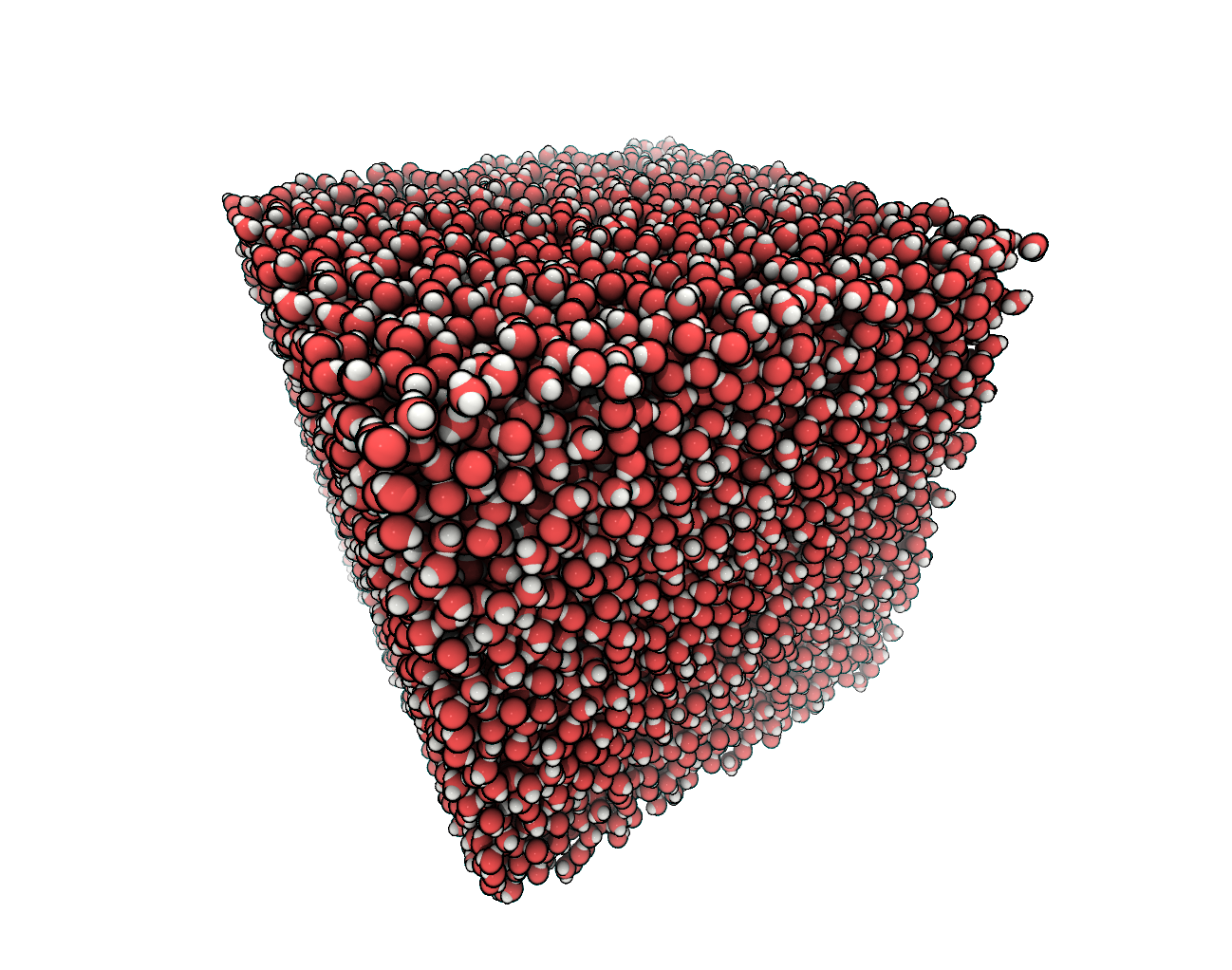
FIGURE We created a cubic simulation box filled with water.
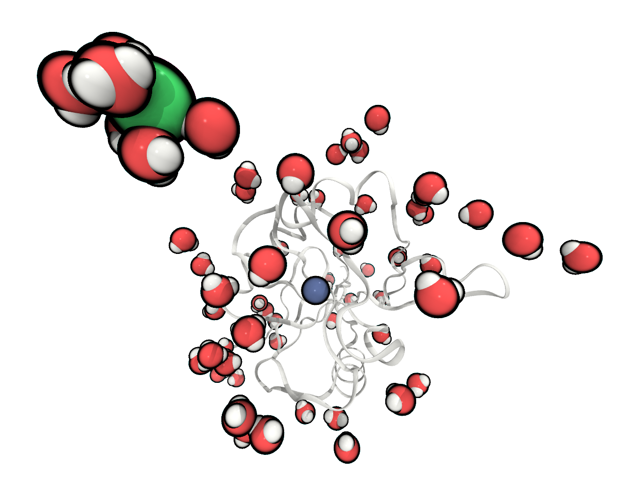
FIGURE The system is fully solvated and one chloride has been added to neutralise the total charge.
Info: In VMD you can add different representation for different atom selection. VMD understand many selection keywords, like "protein", "water", "ion" or "resid 1", "chain A". You can select atoms based on distances (in Å) with e.g. "same resid as within 2 of chain A".
Simulating in OpenMM
Setup
Now that we have our structure well prepared, we can start to use OpenMM for calculations. The standard road to MD simulations usually involves the following steps:
Energy minimisation: The system we have prepared is most probably not in an energy minimum. This is because we have put the solid state crystal structure into a new solvent box, where we removed crystal water and choose solvent positions largely at random. To prevent the system to blow up at the beginning of a simulation, we need to minimise its energy.
NVT equilibration: MD simulations can be performed in different ensembles. Often it is desired to simulate a system under realistic conditions, e.g. say at a physiological temperature. The temperature can be controlled throughout the simulation by coupling the system to a thermostat. When we switch on such a coupling the system needs some time to adjust to it, in other words the temperature needs to equilibrate in a simulation run prior to the actual simulation.
NPT equilibration: If in addition to the temperature also the pressure should be controlled via a barostat, a second equilibration in in which pressure coupling is switched on needs to be done.
Seeding and other optional steps: Once we have a stable equilibrated system, we are good to go for a production MD simulation. In practice other preliminary steps may follow first, like for example a high temperature run to generate a set of starting configurations for a set of production runs.
Although this are the standard steps done to get to the final simulation, depending on the system fewer or more stages can be necessary, like for example a vacuum minimisation before the solvation or several NVT equilibrations under varying conditions.
In any case, OpenMM requires us to setup a system object first, that combines the molecular topology with the chosen force field and simulation parameters. There are different ways to create as system. Here we show using the createSystem method of the force field object created earlier.
[22]:
# Create a simulation system from a force field
system = forcefield.createSystem(
    molecule.topology,                 # pass the molecular topology
    nonbondedMethod=app.PME,           # How to treat non-bonded interactions
    nonbondedCutoff=1*unit.nanometer,  # cutoff for non-bonded interactions
    constraints=app.HBonds             # Constrain H-heavy atom bonds
    )
The system abstracts the molecule in terms of forces considered between its atoms. These forces are calculated during the simulation to propagate the system. Forces are added to the system from the force field according to the topology (e.g. add a harmonic potential for every bond choosing the right force constant). Simulation parameters determine further how to evaluate the different force contribution. PME for example is a scheme used to calculate pairwise electrostatic interactions. We choose a cutoff for the non-bonded interactions of 1 nm beyond which force contributions can be neglected to speed up the simulation. Furthermore, we constraint hydrogen-heavy atom bonds meaning we do not really simulate the corresponding stretching but rather keep the bond lengths at a reasonable value. In this way we can choose a larger time step that does not need to resolve the vibration.
Thermostats and such interacting with the system during the simulation are also considered force contributions, so adding a thermostat for our NVT simulation later is done via the addForce method of the system. We choose an Andersen thermostat with a coupling rate of 1 ps to keep the temperature at 300 K.
[23]:
system.addForce(
    mm.AndersenThermostat(300*unit.kelvin, 1/unit.picosecond)
    )
[23]:
5
We also need to choose an integrator that will actually do the work of calculating forces and modifying atom positions and velocities. Here we use the Verlet integrator and a typical time step of 2 fs.
[24]:
integrator = mm.VerletIntegrator(2.0*unit.femtoseconds)
integrator.setConstraintTolerance(0.00001)
Finally, we have to put everything together once more in another layer of abstraction by creating a simulation object. From this simulation object, the simulations are started later. A simulation bundles the molecular topology (the raw description), the system (the force/parameter description), the integrator (the workhorse), hardware instructions and the simulation context.
[25]:
simulation = app.Simulation(
    molecule.topology,                    # Topology
    system,                               # System
    integrator,                           # Integrator
    mm.Platform.getPlatformByName('CPU')  # Platform
)
Under the term simulation context, OpenMM understands everything that is only secondarily connected to the definition of a simulation, namely the current state of the run with certain atom positions and velocities. In this way, the same conceptual simulation object can run many independent simulations with e.g. different starting structures. We define in the context of our simulation the current molecule positions as starting positions.
[26]:
simulation.context.setPositions(molecule.positions)
Energy minimisation
With having done the abstraction of what and how we want to simulate in a simulation object, minimising the energy is easy.
[27]:
simulation.minimizeEnergy()
After this job is done, we can retrieve the current state of our molecule from the simulation context and save the new atom positions to a file. Let’s see the outcome.
[28]:
state = simulation.context.getState(getPositions=True)
molecule.positions = state.getPositions()
[29]:
with open("min.pdb", "w") as file_:
    molecule.writeFile(
        molecule.topology, molecule.positions,
        file=file_
    )
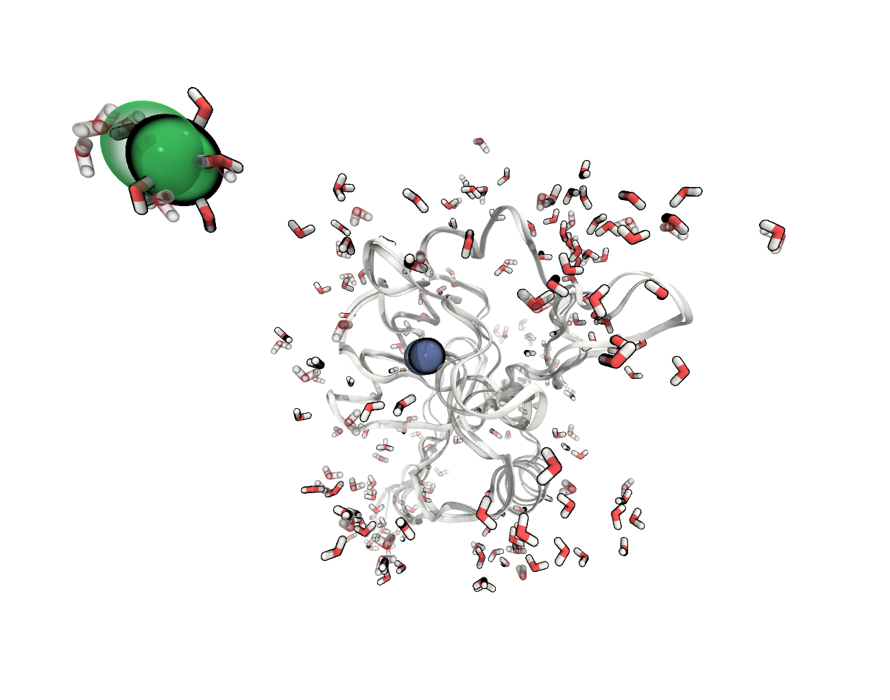
FIGURE The atoms positions in our system have changed during the minimisation (before – transparent).
NVT equilibration
As we can retrieve the context of a simulation, we can in the same way set it whenever we want. Let’s for illustration purposes reload the minimised structure and reset the simulation state.
[30]:
molecule = app.PDBFile("min.pdb")
simulation.context.setPositions(molecule.positions)
Manually getting the state out of a simulation in between runs works fine, but it is also possible to automise this task. OpenMM provides so called Reporters that are attached to a simulation and save data in fixed intervals. When we now want to run a NVT equilibration for 100 ps and we want to save information about the progress of the run and the current temperature every 1 ps, we can do this using a StateDataReporter.
[31]:
run_length = 50000  # 50000 * 2 fs = 100 ps
simulation.reporters.append(
    app.StateDataReporter(
        "equilibration.log", 500, step=True,
        potentialEnergy=True, totalEnergy=True,
        temperature=True, progress=True,
        remainingTime=True, speed=True,
        totalSteps=run_length,
        separator='\t')
        )
Running the simulation for a certain amount of steps is as easy as starting the minimisation. Everything needed for the simulation has been already defined in the simulation object.
[32]:
simulation.step(run_length)
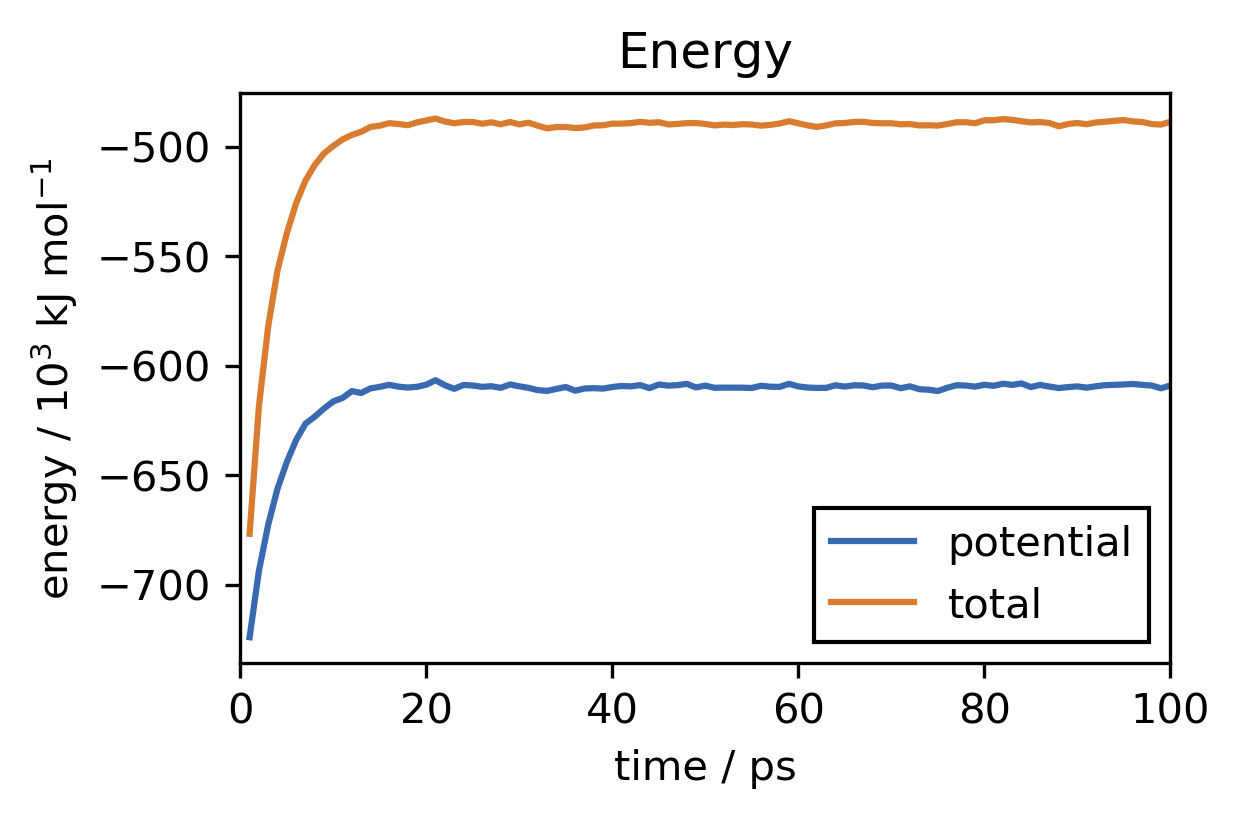
For our system this simulation takes about 1 hour to finish on a reguler 4 CPU core machine. After the simulation has completed we want to check if the equilibration was long enough. We can do this by reading the log-file created by the reporter. We can for example plot the temperature and energy development over time.
[33]:
pot_e = []
tot_e = []
temperature = []

with open("equilibration.log") as file_:
    for line in file_:
        if line.startswith("#"):
            continue
        for l, v in zip((pot_e, tot_e, temperature), line.split()[2:5]):
            l.append(float(v))

t = range(1, 101)
[34]:
plt.close("all")
fig, ax = plt.subplots()
ax.plot(t, [x / 1000 for x in pot_e], label="potential")
ax.plot(t, [x / 1000 for x in tot_e], label="total")

ax.set(**{
    "title": "Energy",
    "xlabel": "time / ps",
    "xlim": (0, 100),
    "ylabel": "energy / 10$^{3}$ kJ mol$^{-1}$"
    })

ax.legend(
    framealpha=1,
    edgecolor="k",
    fancybox=False
)
plt.show()
[35]:
plt.close("all")
fig, ax = plt.subplots()
ax.plot(t, temperature)

ax.set(**{
    "title": "Temperature",
    "xlabel": "time / ps",
    "xlim": (0, 100),
    "ylabel": "temperature / K"
    })
plt.show()
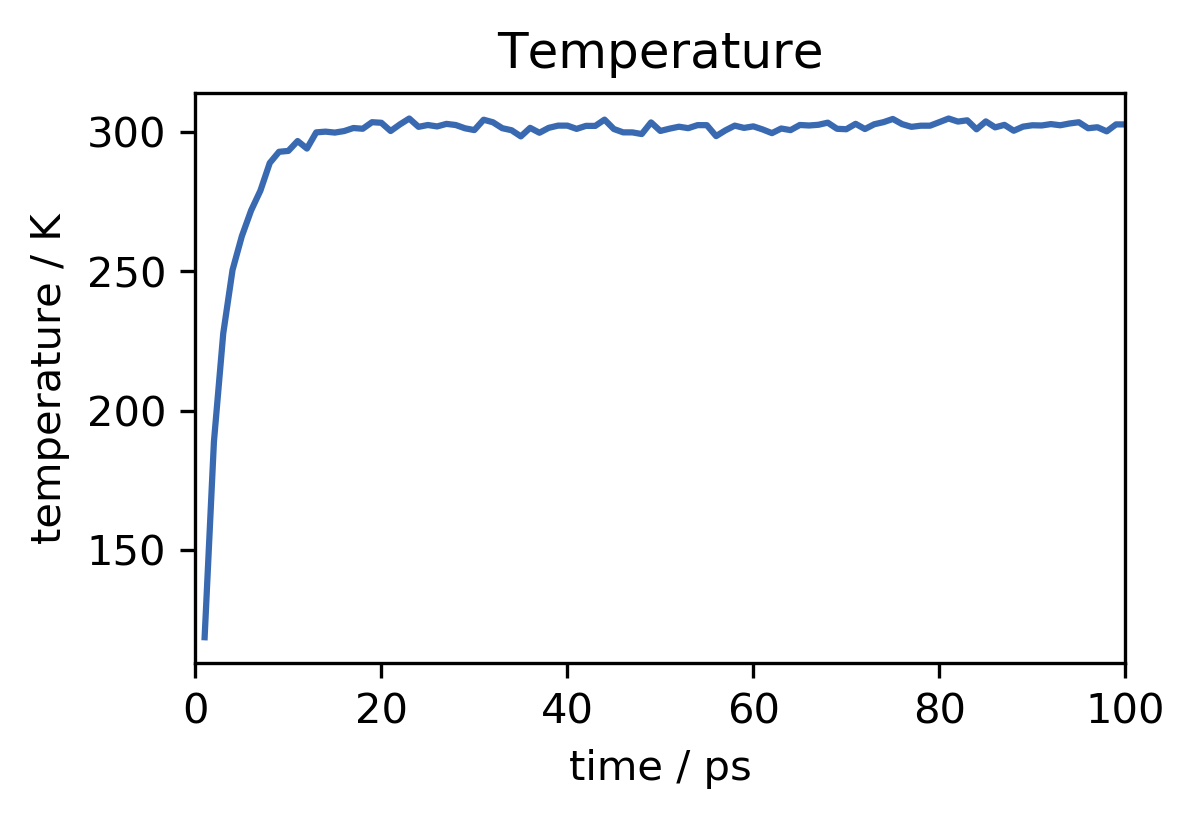
This looks good. In the beginning of the run, the temperature of the system rises from zero (we have started with no initial particle velocities) to the desired value of about 300 K. The observed fluctuations of the instantaneous temperature are expected. Overall temperature and energy are converged well. To save the equilibrated state of the system, including not only atom positions but also velocities and everything that is needed to continue the simulation from here at a later point, we can
instead of accessing the simulation context once more, use the saveState method of the simulation.
[36]:
simulation.saveState("eq.xml")
Production
Continuing from the equilibrated system we could now proceed with a “real” MD simulation. First, we could reload the state into the simulation.
[37]:
simulation.loadState("eq.xml")
Writing output during a simulation is relatively time consuming, so we modify our state reporter that it only writes information to a log-file every 100 ps which is enough to keep track of the progress of the run. We also want to write out the current atom positions in regular intervals to be analysed later as an MD trajectory of atomic coordinates. We could use a PDBReporter for this to append the structures to a PDB file. OpenMM offers, however, also a different format that is better
suited to store long trajectories. A DCDReporter saves positions to a binary .dcd file which uses much less disk space than a .pdb text file. We could for example write out the positions every 10 ps. How long a simulation should be in the end depends much on the question you want to answer with the simulation. If you want to simulate rather slow molecular processes like protein folding you will find yourself quickly in a situation were you would need to simulate several microseconds. The
length of a typical single run may be around a few hundreds of nanoseconds. If we want to simulate our system here for only 100 ns it would take us roughly 40 days to finish this on the machine used for the equilibration, so we will not actually do this now. If you have a GPU with good cooling at your disposal (which can speed up the simulation about a factor of 100) and you do not care too much about your electricity bill, you could give it a try.
[38]:
simulation.reporters = []  # Delete all current reporters

run_length = 50000000  # 50000000 * 2 fs = 100 ns
simulation.reporters.append(
    app.StateDataReporter(
        "simulation.log", 50000, step=True,
        potentialEnergy=True,
        temperature=True, progress=True,
        remainingTime=True, speed=True,
        totalSteps=run_length,
        separator='\t')
    )

simulation.reporters.append(
    app.DCDReporter('trajectory.dcd', 5000)
    )
[39]:
simulation.step(run_length)