Exercise: Molecular Dynamics with OpenMM – Solution

from IPython.core.display import display, HTML
import matplotlib as mpl
import matplotlib.pyplot as plt

import simtk.openmm as mm       # Main OpenMM functionality
import simtk.openmm.app as app  # Application layer (handy interface)
import simtk.unit as unit       # Unit/quantity handling

# Jupyter notebook configuration
display(HTML("<style>.container { width:85% !important; }</style>"))

# matplotlib configuration
mpl.rc_file("../../matplotlibrc")

Inspect the system

Go to the website of the RCSB protein data bank and download the solution NMR structure of a small peptide with the PDB-ID 6a5j as .pdb-textfile. Open the .pdb-file with the text editor of your choice and identify the section in which the molecular structure is described.

• a) How many residues and atoms does the molecule have?

The peptide has 13 residues and 260 atoms.

Ways to find out:

- Inspect the .pdb text file - Load the .pdb file with a molecule viewer (VMD) - Load the .pdb file with OpenMM

molecule = app.PDBFile("md_openmm/6a5j.pdb")
molecule.topology

<Topology; 1 chains, 13 residues, 260 atoms, 259 bonds>

• Parse the .pdb file with Python

with open("md_openmm/6a5j.pdb") as pdbfile:
    print("The structure contains:")
    atom_count = 0   # How many atoms?
    model_count = 0  # How many frames?
    for line in pdbfile:
        if line.startswith("SEQRES"):
            print(f"    {line.split()[3]} residues:")
            print(f"        {' '.join(line.split()[4:])}\n")
            continue
        if line.startswith("MODEL"):
            model_count += 1
            atom_count = 0
            continue
        if line.startswith("ATOM"):
            atom_count += 1
            continue
    print(f"    {atom_count} atoms\n")
    print(f"    {model_count} frames\n")

The structure contains:
    13 residues:
        ILE LYS LYS ILE LEU SER LYS ILE LYS LYS LEU LEU LYS

    260 atoms

    20 frames

• b) Copy the atom definitions for the second amino acid residue and include it in your report.

print_residue = 2
with open("md_openmm/6a5j.pdb") as pdbfile:
    for line in pdbfile:
        if not line.startswith("ATOM"):
            continue
        if int(line[22:26]) < print_residue:
            continue
        if int(line[22:26]) > print_residue:
            break
        print(line.strip())

ATOM     22  N   LYS A   2      -7.295   3.130  -0.024  1.00  0.08           N
ATOM     23  CA  LYS A   2      -6.396   2.084  -0.500  1.00  0.07           C
ATOM     24  C   LYS A   2      -6.593   0.793   0.291  1.00  0.08           C
ATOM     25  O   LYS A   2      -6.656   0.809   1.521  1.00  0.09           O
ATOM     26  CB  LYS A   2      -4.934   2.531  -0.384  1.00  0.08           C
ATOM     27  CG  LYS A   2      -4.546   3.653  -1.334  1.00  0.11           C
ATOM     28  CD  LYS A   2      -3.114   4.126  -1.099  1.00  0.12           C
ATOM     29  CE  LYS A   2      -3.033   5.105   0.061  1.00  0.62           C
ATOM     30  NZ  LYS A   2      -3.301   4.453   1.372  1.00  1.15           N
ATOM     31  H   LYS A   2      -6.928   3.882   0.486  1.00  0.19           H
ATOM     32  HA  LYS A   2      -6.625   1.895  -1.537  1.00  0.09           H
ATOM     33  HB2 LYS A   2      -4.750   2.865   0.626  1.00  0.10           H
ATOM     34  HB3 LYS A   2      -4.298   1.682  -0.589  1.00  0.10           H
ATOM     35  HG2 LYS A   2      -4.633   3.296  -2.350  1.00  0.13           H
ATOM     36  HG3 LYS A   2      -5.218   4.485  -1.184  1.00  0.12           H
ATOM     37  HD2 LYS A   2      -2.484   3.270  -0.879  1.00  0.56           H
ATOM     38  HD3 LYS A   2      -2.756   4.613  -1.994  1.00  0.49           H
ATOM     39  HE2 LYS A   2      -2.043   5.536   0.080  1.00  1.15           H
ATOM     40  HE3 LYS A   2      -3.759   5.890  -0.097  1.00  1.06           H
ATOM     41  HZ1 LYS A   2      -2.685   3.624   1.493  1.00  1.67           H
ATOM     42  HZ2 LYS A   2      -4.292   4.147   1.422  1.00  1.71           H
ATOM     43  HZ3 LYS A   2      -3.118   5.123   2.147  1.00  1.58           H

Open the .pdb-file in VMD.

• c) How many structures are contained in the file?

The .pdb-file contains 20 structures.

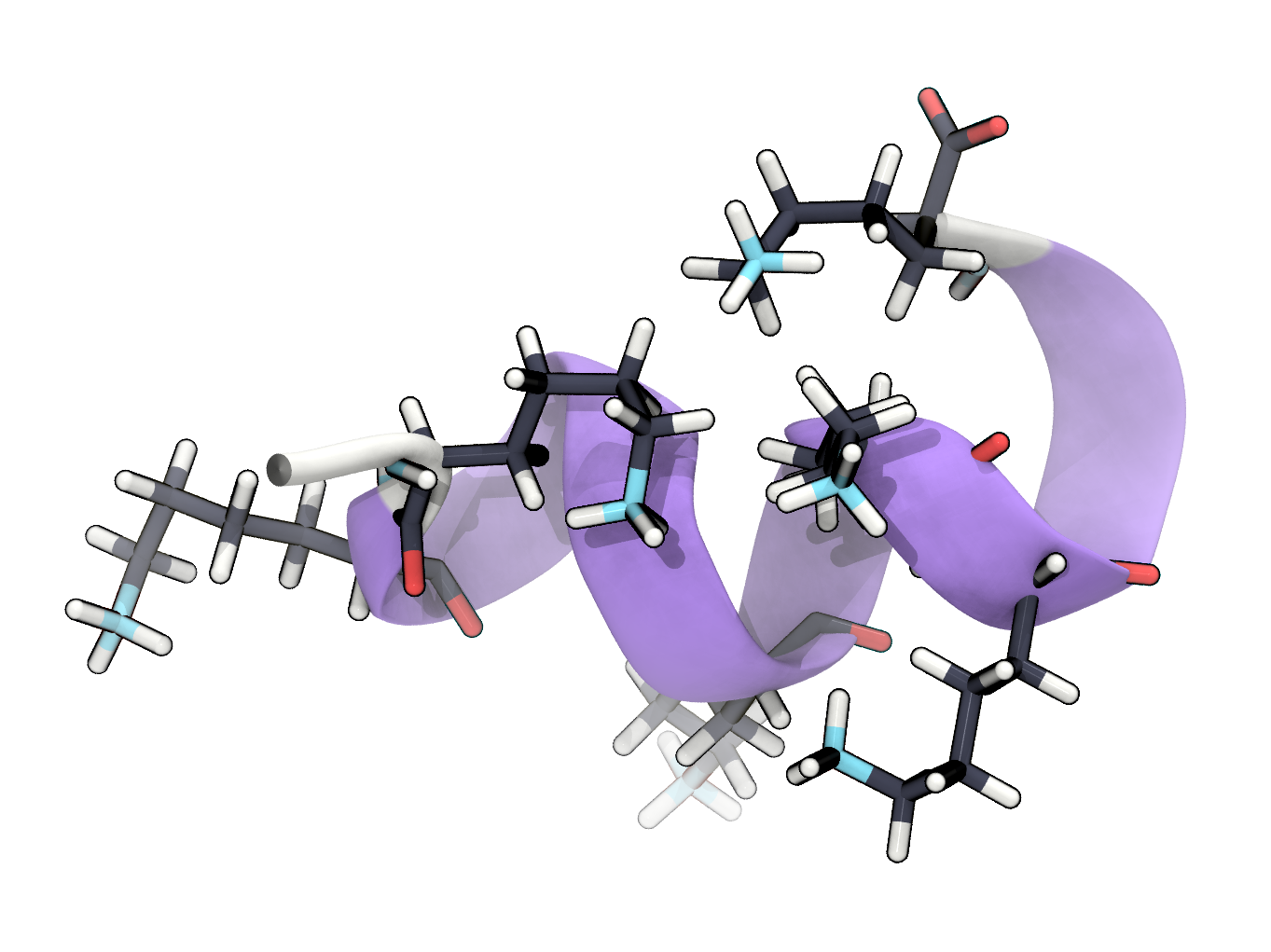
• d) Set the background colour to white and remove the axis icon. Visualise the peptide structure in a representation that emphasises the secondary structure (e.g. NewCartoon, NewRibbons, …) and choose Secondary Structure as colouring method. Visualise the side chain of lysines in the structure in a representation that shows bonds and atoms (e.g. Licorice, CPK, …) and color them by chemical element. Render an image of the first structure frame and include it in your report.

• e) The structure file contains hydrogens. What is the total charge of the peptide?

Rational approach The peptide has 6 lysine residues in its sequence. All lysine side chains are protonated and the total charge of the molecule is +6.

Forcefield approach Get the total charge of the system from the partial charges of the atoms:

forcefield = app.ForceField("amber14/protein.ff14SB.xml")
system = forcefield.createSystem(molecule.topology)

for force in system.getForces():
    print(type(force))
    if isinstance(force, mm.openmm.NonbondedForce):
        # For charges, we are only interested in the non-bonded forces
        nonbonded = force

<class 'simtk.openmm.openmm.HarmonicBondForce'>
<class 'simtk.openmm.openmm.HarmonicAngleForce'>
<class 'simtk.openmm.openmm.PeriodicTorsionForce'>
<class 'simtk.openmm.openmm.NonbondedForce'>
<class 'simtk.openmm.openmm.CMMotionRemover'>

A non-bonded force entry of an atom looks like this:

nonbonded.getParticleParameters(0)

[Quantity(value=0.0311, unit=elementary charge),
 Quantity(value=0.3249998523775958, unit=nanometer),
 Quantity(value=0.7112800000000001, unit=kilojoule/mole)]

force_description = zip(
    ["Partial charge", "Minimum energy distance", "Minimum energy"],
    nonbonded.getParticleParameters(0)
)

for desc, comp in force_description:
    print(f"{desc:<26} {comp}")

Partial charge             0.0311 e
Minimum energy distance    0.3249998523775958 nm
Minimum energy             0.7112800000000001 kJ/mol

total_charge = 0.
for i in range(nonbonded.getNumParticles()):
    nb_i = clePnonbonded.getPartiarameters(i)
    total_charge += nb_i[0].value_in_unit(unit.elementary_charge)
total_charge

5.999999999999995

round(total_charge)

6

Prepare the structure

Save the first structure included in the .pdb-file to a new separate .pdb file, e.g. conf.pdb. We want to use this frame as starting structure for our simulation. Use OpenMM to load the structure into memory.

Ways to achieve this:

- Copy the ATOM entries for MODEL 1 manually to a new file - Use File > Save Coordinates dialog in VMD - Parse the file with Python

with open("md_openmm/6a5j.pdb") as pdbfile:
    with open("md_openmm/conf.pdb", 'w') as newfile:
        model_count = 0
        for line in pdbfile:
            if line.startswith("MODEL"):
                model_count += 1
                if model_count > 1:
                    break
                continue
            if not line.startswith("ATOM"):
                continue
            newfile.write(line)

molecule = app.PDBFile("md_openmm/conf.pdb")

• a) Investigate the topology attribute of the loaded molecule. How many covalent bonds are present?

print(molecule.topology)

<Topology; 1 chains, 13 residues, 260 atoms, 259 bonds>

• b) We want to simulate the molecule using the AMBER 14SB force field in TIP3P water. Create a forcefield object suitable for this purpose.

forcefield = app.ForceField(
    "amber14/protein.ff14SB.xml",
    "amber14/tip3p.xml"
)

• c) Our structure file does not include solvent and has a non-zero total charge. Put the molecule in a cubic water box with a minimum distance of 1 nm to the box boarders. Make sure that also counter ions are added to neutralise the system.

model = app.Modeller(molecule.topology, molecule.positions)
model.addSolvent(
    forcefield,
    padding=1 * unit.nanometer,
    neutralize=True
    )

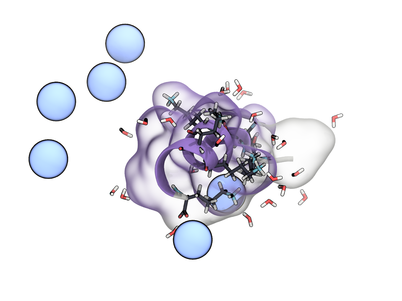
• d) Save the modified structure (peptide plus solvent and ions) to a .pdb-file. Load the structure into VMD and visualise the peptide as before. Additionally show ions as van-der-Waals spheres and water molecules within a distance of 2 Å in the Licorice representation. Optional Add a transparent surface representation (e.g. QuickSurf) for the peptide.

molecule.positions = model.getPositions()
molecule.topology = model.getTopology()

with open("md_openmm/solv.pdb", "w") as file_:
    molecule.writeFile(
        molecule.topology, molecule.positions,
        file=file_
    )

Simulation

Setup

• a) Create a system object from the topology of the solvated peptide with the forcefield you setup earlier. Use H-bonds constraints, and PME for nonbonded interactions (cutoff 1 nm).

molecule = app.PDBFile("md_openmm/solv.pdb")

system = forcefield.createSystem(
    molecule.topology,
    nonbondedMethod=app.PME,
    nonbondedCutoff=1 * unit.nanometer,
    constraints=app.HBonds
    )

• b) We want to simulate in the NVT ensemble. Add an Andersen thermostat to the system to keep the temperature at 300 K (coupling rate 1/ps).

system.addForce(
    mm.AndersenThermostat(300 * unit.kelvin, 1 / unit.picosecond)
    )

5

• c) We want to propagate the simulation using a Verlet integrator in timesteps of 2 fs (we need a contraint tolerance of 0.00001). Setup a simulation object with the solvated topology, the system and the integrator. Use "CPU" as the simulation platform.

integrator = mm.VerletIntegrator(2.0*unit.femtoseconds)
integrator.setConstraintTolerance(0.00001)

simulation = app.Simulation(
    molecule.topology,                    # Topology
    system,                               # System
    integrator,                           # Integrator
    mm.Platform.getPlatformByName('CPU')  # Platform
)

How to figure out which platform to use?

n_platforms = mm.Platform.getNumPlatforms()  # How many platforms are supported?
n_platforms

2

for i in range(n_platforms):
    print(mm.Platform.getPlatform(i).getName())

Reference
CPU

• d) Add the current atomic positions of the solvated peptide to the context of the simulation.

simulation.context.setPositions(molecule.positions)

Energy minimisation

• a) Minimise the energy of the system. Save the new positions to a .pdb-file.

simulation.minimizeEnergy()

state = simulation.context.getState(getPositions=True)
molecule.positions = state.getPositions()

with open("md_openmm/min.pdb", "w") as file_:
    molecule.writeFile(
        molecule.topology, molecule.positions,
        file=file_
    )

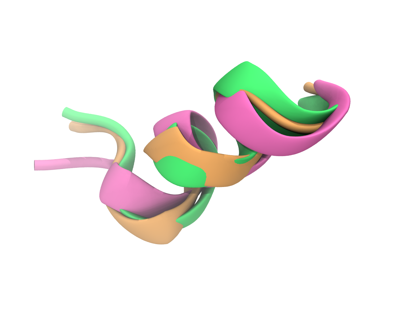
• a) Open the structure in VMD and render an image the same way as in the last step in which the original and the minimised atoms are overlaid. Choose different colors for the two states. Can you see the difference?

Equilibration

• a) We now want to equilibrate our system in the NVT ensemble for 100 ps. Add a state reporter to the simulation object that reports the total and potential energy and the temperature at every picosecond and write it to a file (e.g. equilibration.log).

molecule = app.PDBFile("md_openmm/min.pdb")
simulation.context.setPositions(molecule.positions)

run_length = 50000  # 50000 * 2 fs = 100 ps
simulation.reporters.append(
    app.StateDataReporter(
        "md_openmm/equilibration.log", 500, step=True,
        potentialEnergy=True, totalEnergy=True,
        temperature=True, progress=True,
        remainingTime=True, speed=True,
        totalSteps=run_length,
        separator='\t')
    )

• b) Run the simulation. It should take about 10 minutes to complete on a processor with 4 cores. Reduce the number of steps, if it takes much longer on your hardware.

simulation.step(run_length)

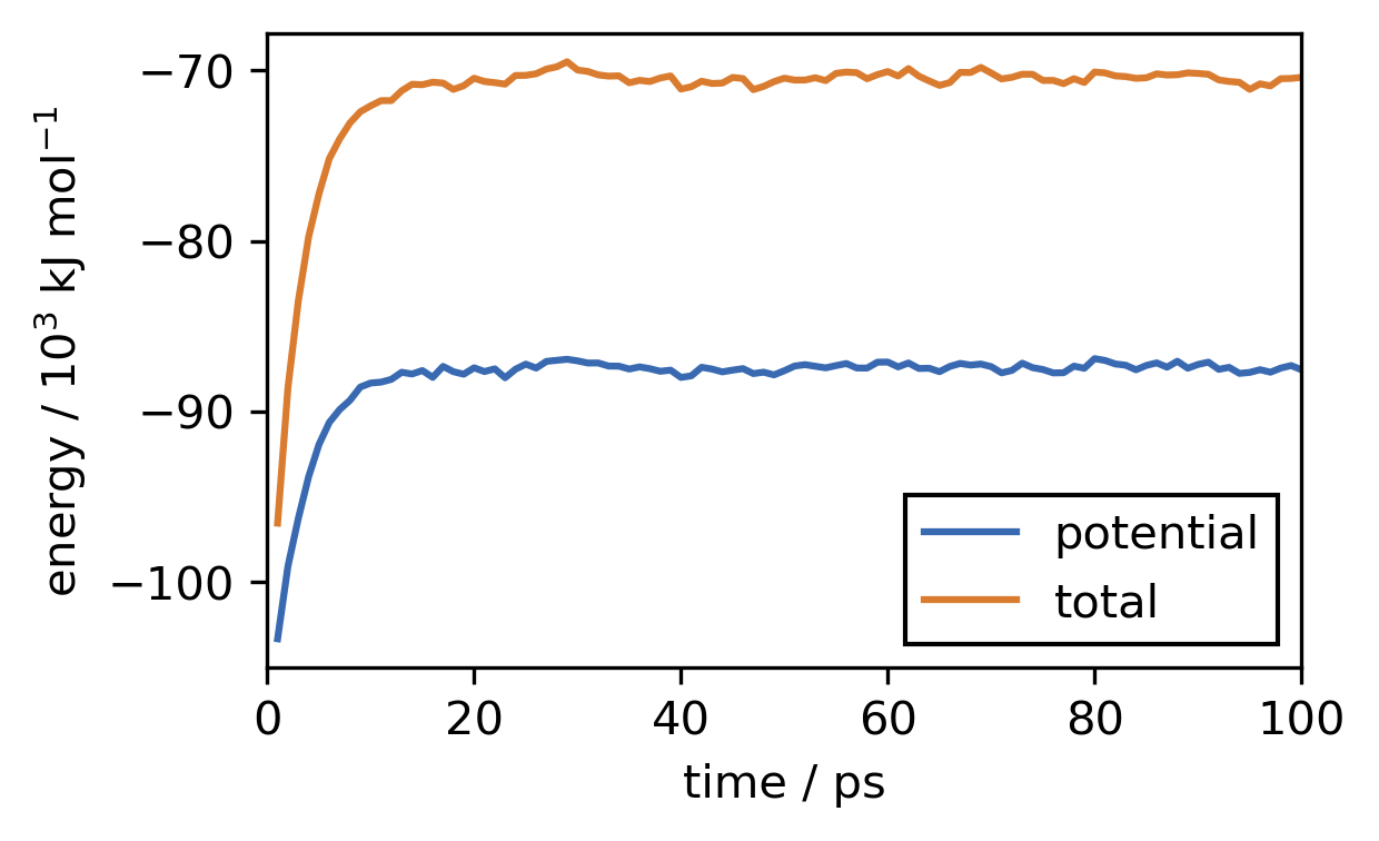
• c) Plot the energies against the simulation time step.

pot_e = []
tot_e = []
temperature = []

with open("md_openmm/equilibration.log") as file_:
    for line in file_:
        if line.startswith("#"):
            continue
        pot_e_, tot_e_, temperature_ = line.split()[2:5]
        pot_e.append(float(pot_e_))
        tot_e.append(float(tot_e_))
        temperature.append(float(temperature_))

        # Alternative solution:
        # for l, v in zip((pot_e, tot_e, temperature), line.split()[2:5]):
        #     l.append(float(v))

t = range(1, 101)

fig, ax = plt.subplots()
ax.plot(t, [x / 1000 for x in pot_e], label="potential")
ax.plot(t, [x / 1000 for x in tot_e], label="total")

ax.set(**{
    "xlabel": "time / ps",
    "xlim": (0, 100),
    "ylabel": "energy / 10$^{3}$ kJ mol$^{-1}$"
    })

ax.legend(
    framealpha=1,
    edgecolor="k",
    fancybox=False
)

<matplotlib.legend.Legend at 0x7f07884e3080>

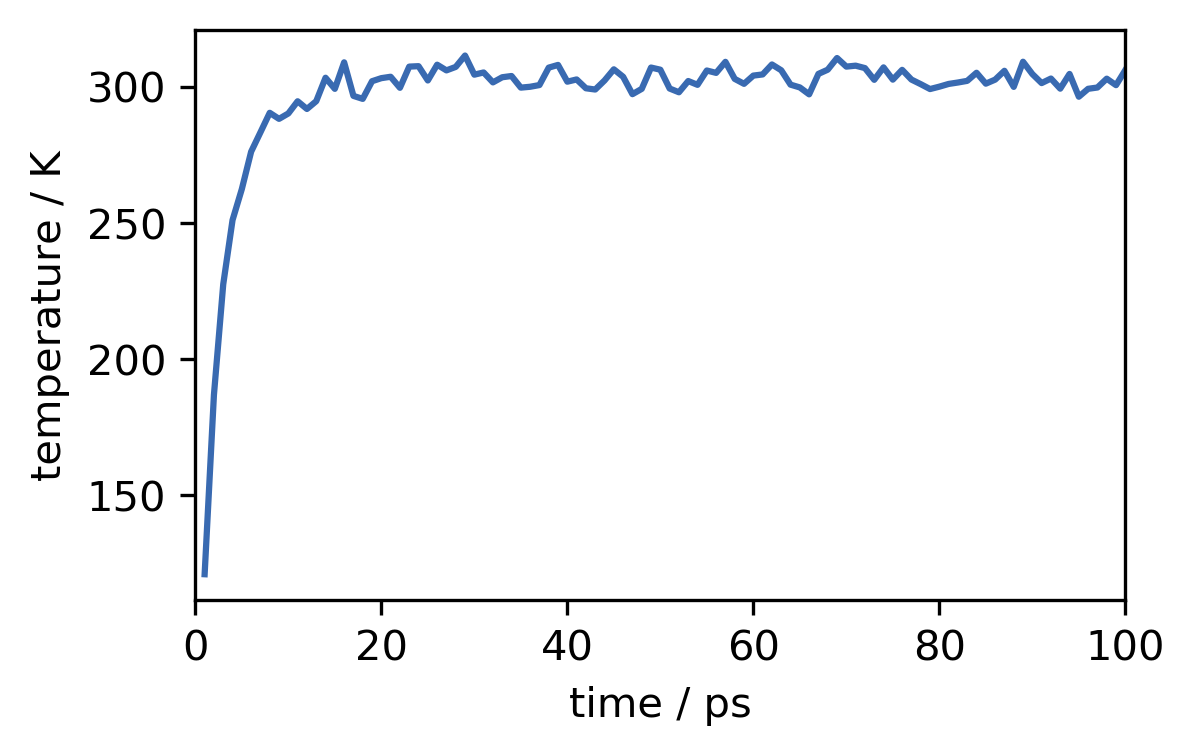
• d) Plot the temperature against the simulation time step.

fig, ax = plt.subplots()
ax.plot(t, temperature)

ax.set(**{
    "xlabel": "time / ps",
    "xlim": (0, 100),
    "ylabel": "temperature / K"
    })

[Text(0, 0.5, 'temperature / K'), (0, 100), Text(0.5, 0, 'time / ps')]

• e) Save the current state of the simulation to an .xml-file.

simulation.saveState("md_openmm/eq.xml")

Production

• a) Load the state of the equilibrated system into the simulation object.

simulation.loadState("md_openmm/eq.xml")

• b) Reset the simulation reporters. Let’s now assume we want to simulate the system for 100 ns. Add a state reporter to the simulation object that reports the potential energy every 10 ps and writes it to a file (e.g. simulation.log). Add a structure reporter that saves the current atom positions to a .pdb-file every 10 ps.

simulation.reporters = []

run_length = 50000000  # 50000000 * 2 fs = 100 ns
simulation.reporters.append(
    app.StateDataReporter(
        "md_openmm/simulation.log", 5000, step=True,
        potentialEnergy=True,
        temperature=True, progress=True,
        remainingTime=True, speed=True,
        totalSteps=run_length,
        separator='\t')
    )

simulation.reporters.append(
    app.PDBReporter('run.pdb', 5000)
    )

• c) The simulation can easily take several days to finish, depending on the used hardware, so you do not have to run it yourself completely. Just start the simulation to see if everything works and run it until the first structure has been saved by the structure reporter (after 10 ps).

simulation.step(5100)

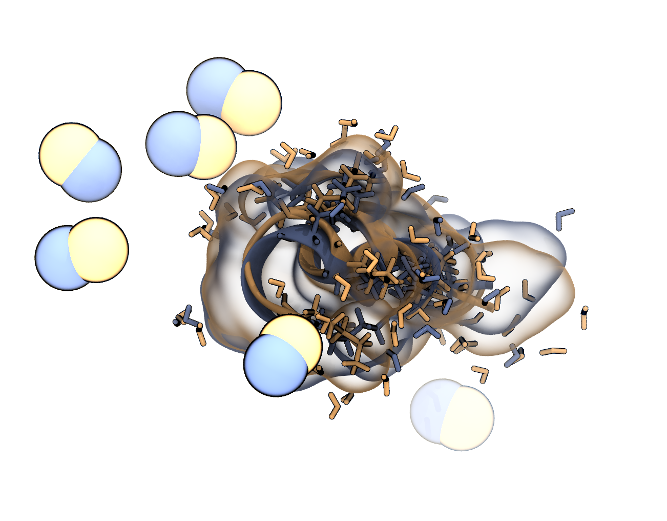
• d) Open the saved .pdb-file in VMD. Render an image that shows only the peptide in a representation which emphasises the secondary structure and compares the original to the minimised and the current conformation. Align the structures (e.g. using the RMSD Trajectory Tool).